Back to Home
← All guides

Microscopy · 20 min

How to choose a laser for microscopy

Your fluorophores pick the wavelengths, and that is the easy half. The modality picks everything else — how much power actually has to arrive, how fast the beam has to switch, how the light is delivered, and whether laser noise reaches the image at all.

Power by modalityExcitation linesModulation bandwidthPhototoxicityShot-noise crossover

Start here

Watts are the least interesting number on the quote.

Almost every microscopy laser enquiry arrives as a wavelength and a power. The wavelength is usually right, because it follows directly from the fluorophore panel. The power is usually wrong, and it is wrong in both directions: too much for a confocal, too little for localisation microscopy, and quoted at the laser aperture rather than at the specimen where it means something.

The reason is that the same laser illuminates wildly different areas depending on what the microscope does with it. A widefield field of view is roughly two hundred thousand times larger than a diffraction-limited focus. That single geometric fact is why a point-scanning confocal is comfortable with microwatts at the sample while a STORM experiment on a field a quarter the size needs a hundred milliwatts of the same colour.

So the useful sequence is: fluorophores give you the lines; the modality gives you the irradiance you need and therefore the power; the scanner gives you the modulation specification; the sample gives you the dose you are allowed; and only then — if the photon counts are high enough for it to matter — does the noise specification enter. Most enquiries stop at step one.

The four things that actually constrain you

None of them is the number of milliwatts.

The illuminated area spans five decades

A 200 µm widefield field is about 3×10⁻⁴ cm². A diffraction-limited focus at 488 nm through a 1.4 NA objective is about 1.4×10⁻⁹ cm². That is a factor of 200 000 in area for the same laser, which is why a point scanner is happy with microwatts and a localisation experiment needs half a watt of the same colour.

Saturation caps what power can buy

A fluorophore cannot emit faster than its excited-state lifetime allows. Once the excitation rate approaches 1/τ — a few times 10⁸ s⁻¹ for a typical dye — additional power produces no additional signal, only additional bleaching and photodamage. Point scanners routinely operate within a factor of ten of this ceiling.

Dwell time sets the modulation spec

A confocal running a 2 µs pixel dwell needs the beam to settle in well under a pixel. At a tenth of the dwell, that is a 200 ns transition and roughly 2 MHz of bandwidth. No mechanical shutter does this, and no DPSS laser does it by current control — which is exactly why AOTFs exist in every scan head.

Coherence helps and hurts, depending

Structured illumination needs interference across the whole field, so it wants a long coherence length and stable polarisation. Widefield wants the opposite: a single-frequency source turns every dust particle and every optical surface into a fringe pattern printed on your data. The same specification is a virtue in one modality and a defect in the next.

At a glance

Eight modalities, eight different lasers.

Same fluorophores, same objective, same detector — and a two-hundred-fold spread in the power you have to buy, plus completely different demands on how the beam is switched and delivered. Find your row before you read anything else on this page.

ModalityIrradiance at the samplePower at the fibreSwitchingWhat actually decides the choice
Widefield epifluorescence0.1–10 W/cm²5–50 mW per lineShutter, millisecondsField uniformity and freedom from speckle. Power is almost never the constraint.
Spinning-disk confocal10–100 W/cm²50–500 mW per lineMillisecond gatingPower surviving the pinhole array — the disk itself typically passes only a few percent.
TIRF100–1 000 W/cm²20–100 mW per lineMilliseconds, per channelPolarisation stability and a clean single-mode beam. PM fibre is not optional.
Light-sheet1–50 W/cm²20–200 mW per linePer-plane gatingM² and pointing — the sheet thickness is set by the beam quality, not by the laser power.
Point-scanning confocal1–10 kW/cm²10–50 mW per lineAOTF or direct, ≥ 1 MHzModulation bandwidth against pixel dwell time. Microwatts reach the sample.
SMLM (STORM / PALM)1–10 kW/cm²300 mW – 1 W at 640 nmGating plus a ramped 405 nm activation lineRaw power, and independent control of the activation channel.
Two-photonGW/cm² peak, 1–20 mW average at the sample0.5–3 W at the objective for depthFemtosecond, ~80 MHzPulse width surviving to the focus, and tunability across the two-photon cross sections.
FLIM / TCSPCAs the scanning modality it sits on1–50 mW pulsed20–80 MHz pulsed, low jitterPulse width and timing jitter — together they are your instrument response function.

Irradiance figures are the ranges in routine use rather than hard limits, computed from the field or focus area each modality illuminates. Power at the fibre assumes roughly 30 % throughput to the specimen. STED is omitted from the table because its depletion beam is a separate design problem: it needs watt-class power at 592, 660 or 775 nm, a phase mask, and either picosecond synchronisation to the excitation pulse or a CW depletion scheme.

Interactive

Work out the power you actually need.

Set the modality, the line, the fluorophore and the objective, and the chain from irradiance to detected photons is computed end to end. Two things usually surprise people: how little power a scanner needs, and how completely the excitation efficiency of an off-peak line dominates the arithmetic.

Photon budget lab

From power at the sample to photons in the pixel

Pick the modality first. The illuminated area changes by five orders of magnitude across this list, and it is the single reason the same fluorophore needs microwatts on one microscope and half a watt on another.

Imaging modality

All the power sits in one diffraction-limited focus for a few microseconds. Microwatts at the sample already produce kilowatts per square centimetre.

Peak 488 nm · ε 55,900 M⁻¹cm⁻¹ · QY 0.6 · τ 2.6 ns

5.00 µW

After the objective. Expect to lose 60–80 % between the fibre tip and here.

2.0 µs

How long each molecule sits in the focus. This sets the modulation bandwidth the laser needs.

Focal spot

210 nm radius

Airy radius 0.61λ/NA. A scanner has no field-size slider — the objective sets the area.

100 molecules

1 for single-molecule work, 10–100 for a sparse tag, 10³–10⁴ for a bright structural stain.

Irradiance at the sample

3.62 kW/cm²

Over 1.38e-9 cm²

Excitation efficiency

100 %

488 nm against a 488 nm peak

Saturation of the dye

0.492 %

Fraction of time the molecule is already excited

Collection efficiency

32.3 %

NA 1.42 in n = 1.518

Detected per molecule

0.21

photons per dwell

Detected per spot

21

100 molecules together

Shot-noise-limited SNR in this pixel

4.6 : 1

Usable but thin. You can see structure and you cannot measure it. Either raise the dose, lengthen the exposure, or accept binning — and note that only one of those three costs you photobleaching.

Frames before the dye is spent

17,632

Assuming a total budget of 4×10⁴ emitted photons per molecule and strictly linear bleaching. Real bleaching accelerates faster than linearly above roughly a kilowatt per square centimetre, so treat this as an optimistic ceiling.

Required at the fibre tip

17 µW

At 30 % end-to-end throughput, which is a realistic number for an AOTF, a scan head, a dichroic and an objective in series. Specify the laser against this figure, never against the power at the sample.

What the numbers say about the laser

You are deep in the shot-noise-limited regime. With 21 detected photons, photon statistics alone contribute 21.6 %, which buries any amplitude noise a real laser produces. Buy stability and modulation, not a low-RIN premium.

Excitation spectra are approximated as split Gaussians about the published absorption peak, wide to the blue and narrow to the red. That reproduces the shape and the asymmetry of a real spectrum but not its vibronic detail — for a final design, use the measured spectrum of the exact fluorophore in the exact buffer. Emission-side transmission is fixed at 65 % for the objective, dichroic, emission filter and tube lens together.

The easy decision

Which lines, and what each one costs you.

The standard four-colour panel is 405, 488, 561 and 640 nm, and it exists because those four lines cover the overwhelming majority of commercial fluorophores while staying far enough apart for filter sets to separate them. What the panel does not tell you is that the four are not equally cheap in dose.

405 nm

DAPI, Hoechst, BFP; photoactivation of PA-GFP and PS-CFP; mEos photoconversion

The most phototoxic line in routine use and the one that lifts cellular autofluorescence hardest. In SMLM it is an activation control, not an imaging channel — microwatts, ramped under software.

445 / 450 nm

CFP, mTurquoise2, and the donor half of most FRET pairs

Useful when 405 nm is too damaging and 488 nm crosstalks into the acceptor. Cheap and widely stocked as a direct diode.

488 nm

GFP, EGFP, FITC, Alexa Fluor 488, GCaMP

The workhorse, and also where flavin autofluorescence peaks. If your background is stubborn and your dye choice is free, the same experiment in the red usually has a cleaner floor.

514 / 520 nm

YFP, Venus, Citrine

Buys you spectral separation from GFP that 488 nm cannot, which is what makes a GFP–YFP FRET pair workable.

532 / 552 / 561 nm

mCherry, tdTomato, TRITC, Alexa Fluor 555 and 568, mRFP

561 nm sits far closer to the red-protein absorption peaks than 532 nm does. 532 nm is cheaper and available at much higher power, but on mCherry it works at roughly half the efficiency.

594 nm

Texas Red, Alexa Fluor 594, mKate2, mScarlet

The line that separates a red channel from an orange one. Frequently the missing channel in a four-colour panel built around 405/488/561/640.

633 / 637 / 640 nm

Cy5, Alexa Fluor 647, ATTO 647N, SiR dyes, DRAQ5

The cleanest and gentlest of the standard panel: lowest autofluorescence, lowest phototoxicity per photon, and the brightest dyes in the catalogue. The default STORM channel for good reason.

730 / 750 nm

Alexa Fluor 750, Cy7, and NIR-I multiplexing labels

A fifth or sixth colour, and the least damaging of all. Detector QE falls away here, so budget photons rather than assuming the red trend continues for free.

The constraint nobody writes on the purchase order

You are not buying photons. You are spending a dose budget.

Photobleaching and phototoxicity share a mechanism. Both are driven largely by reactive oxygen species generated from the fluorophore triplet state, so both scale with the number of excitation cycles — the same quantity that produces your signal. Every photon you collect is spent from a finite budget, and the budget belongs to the sample, not to the laser.

Two results from the live-imaging literature change how you specify a source. The first is that damage falls steeply toward the red: cells irradiated at 640 nm tolerate far more energy than the same cells at 405 nm. The second is less intuitive and more useful — for the same total dose, spreading it over a longer, gentler exposure is less damaging than a short intense burst, because triplet accumulation and higher-order absorption are superlinear in intensity.

Put together, those two rules say something specific about the purchase: prefer the reddest line your labels allow, prefer a source you can turn down smoothly and accurately under analog control, and treat any request for more power as a question about the detector first.

The second decision

How fast the beam has to switch.

For a camera-based microscope this barely matters — a millisecond shutter is fine when the exposure is fifty. For anything scanned it is the specification that decides whether the laser is usable at all, and it is the reason microscopy sources cost what they do.

Start from the dwell time

f₃dB ≈ 0.35 / t_rise, t_rise ≲ t_dwell / 10

A 2 µs pixel dwell allows a 200 ns transition if the edge is not to smear into the neighbouring pixel, which asks for roughly 2 MHz. Slower than that and your blanking during flyback leaves a bright stripe down one side of the frame.

Direct modulation, and its price

diode: ns DPSS: τ_upper ≈ 10–300 µs

A diode follows its current in nanoseconds, so it modulates directly — but the wavelength chirps with current and the mode structure changes near threshold. A DPSS laser stores energy in a crystal and answers a current step with relaxation oscillations, so it cannot be switched cleanly at all.

Which is why AOTFs exist

t_rise ≈ d_beam / v_acoustic

An acousto-optic device switches as fast as sound crosses the beam. Slow-shear TeO₂ carries sound at about 617 m/s, so a 1 mm beam gives 1.6 µs and a 100 µm beam gives 160 ns. A switching specification without the beam diameter it was measured at means nothing.

Ask for analog, not just TTL

TTL gating gets you on and off, which covers blanking and per-channel sequencing. It does not get you a photoactivation ramp, a bleach pulse at a controlled fraction of full power, or per-line intensity adjustment inside a z-stack — all of which need the beam set to an arbitrary level, quickly and repeatably.

The other number to ask for is extinction in the off state. An AOTF typically blanks to around 1000:1, which is fine for scanning and not fine for a FRAP experiment where the residual beam keeps bleaching the region you are watching recover. Where that matters, put a mechanical shutter in series and accept the millisecond.

Pulsed sources are a different question

FLIM needs pulses short against the lifetime you are measuring and a repetition period long enough for the excited state to decay between them. A 4 ns lifetime wants roughly 20 MHz rather than 80, and the pulse width plus the timing jitter together are your instrument response function — quote both.

Two-photon depends on the square of the instantaneous intensity, so it lives entirely on peak power. Ten milliwatts average in 100 fs pulses at 80 MHz is about 1.25 kW peak — five orders of magnitude above the same average power delivered continuously. Watch the dispersion budget too: every lens between the laser and the focus stretches the pulse, and a stretched pulse is a dimmer image at the same average power.

Interactive

When does laser noise reach the image?

“Low noise” is the most abused phrase on a laser datasheet, and in microscopy it is usually irrelevant — because fluorescence pixels are starved of photons and shot noise buries everything else. There is a specific photon count above which that stops being true, and it is worth knowing which side of it you are on before you pay for the premium.

Noise crossover lab

Does laser noise reach your image at all?

Shot noise falls as the signal grows. Laser amplitude noise does not. Where the two lines cross is the only place a low-RIN premium starts buying you anything.

Typical measurements

3,000 photons

One pixel, or a whole region of interest if that is what you actually quantify.

0.50 %

Catalogue diode and DPSS heads quote 0.5–1 %. Ask which band the figure covers.

1×

Averaging suppresses shot noise and in-band laser noise equally. It does nothing to drift.

1.0 %

The 4-hour or 8-hour stability figure on the datasheet, over the length of your session.

10¹10²10³10101010100 %10 %1 %0.1 %0.01 %crossoverdetected photons
shot noise laser noise floor combined

Shot noise

1.83 %

1/√N, after averaging

Laser noise

0.500 %

in band, after averaging

Combined random error

1.89 %

4 % worse than shot-limited

Crossover

40,000

photons, where the two are equal

Verdict

Shot-noise limited with room to spare: the laser adds about 4 percent to the total error. You would need 40,000 photons before a 0.50 % source became the limitation. Specify stability and modulation instead, and spend the saved money on the objective and the detector.

Drift is separate and does not average. A 1.0 % drift over the session is a 1.0 % systematic error between the first frame and the last, no matter how many photons you collect or how many frames you average. On the numbers above it is 0.5× the random error. For time-lapse intensity work, ratiometric imaging, or anything compared across a session, this is the specification that actually decides the result.

Read noise, dark current and background fluorescence are omitted; each adds its own term in quadrature and moves the crossover to the right, so this chart is the optimistic case for the laser mattering. In-band noise is treated as white across the averaging window, which is fair above a few hertz and optimistic below it, where 1/f dominates.

Beam delivery

The fibre decides more than the laser does.

Once a source is fibre-coupled, its M² and pointing specifications stop being visible to you. What you get instead is the fibre mode, and choosing it wrongly produces artefacts that no amount of laser quality fixes.

Single-mode

A clean Gaussian, perfectly repeatable, alignment-free at the microscope end. The cost is that a Gaussian is not a flat field: illuminate a 200 µm field with the central part of a Gaussian and the corners see materially less light than the centre unless you expand and clip, which throws away most of the power. Fine for scanning, awkward for quantitative widefield without a beam shaper or a flat-field correction.

Polarisation-maintaining

Everything single-mode fibre gives you, plus a polarisation state that survives the room warming up. TIRF depth uniformity, SIM pattern contrast, and any anisotropy measurement all depend on it. Ordinary SM fibre rotates the state slowly with temperature and stress, and the resulting drift looks exactly like the sample changing.

Multimode

More power, more forgiving coupling, and a more uniform field — with speckle, unless the mode content is scrambled faster than your exposure. A vibrating fibre or a rotating diffuser turns speckle into a uniform average. The requirement is that the scrambling runs faster than the frame, not faster than your eye.

Coherence length is a two-sided specification

L_c ≈ λ² / Δλ

A single-frequency 561 nm laser with a 1 MHz linewidth has a coherence length of hundreds of metres, so every optical surface in the path becomes an etalon and every scatterer produces speckle. A multimode diode at 640 nm with a 1 nm spectral width has a coherence length of about 0.4 mm — short enough that most fringing simply disappears.

For widefield and light-sheet, the broader source is the better buy, which is one of the few places in optics where the worse-looking specification wins. Structured illumination is the clear exception: SIM builds its pattern by interference across the field, so it needs the coherence kept and the polarisation controlled.

Where fibre-coupled stability really comes from

On a free-space head, pointing drift moves your beam. On a fibre-coupled head it does something less obvious and more damaging: it moves the beam relative to the fibre core, and the coupled power changes. A launch that is 80 % efficient and drifts by a micrometre can lose several percent of transmitted power without the laser itself changing at all.

This is why the stability figure quoted after the fibre is the one that matters, and why it is usually worse than the figure at the aperture. Ask which side of the fibre the number was measured on. A supplier who has measured both is telling you something real about how the product was built.

The specification sheet

Seven numbers to demand, and what each one protects.

Power at the fibre output, per line

Three times your computed requirement at the sample

Corrupts: Every dose calculation you make

Datasheets quote power at the laser aperture. Between there and the specimen sit an AOTF, a fibre launch, a scan head, a dichroic and an objective. Thirty percent end-to-end is a fair working assumption and twenty is common, so a 30 mW line is a 6–10 mW line where it counts.

Power stability over the session (%)

< 1 % over 8 h; < 0.5 % if you publish intensities

Corrupts: Time-lapse intensities, ratios, and any comparison between conditions

Drift is a pure systematic. It survives every frame you average and every pixel you bin, and it is indistinguishable from the biology getting brighter. It is the specification that decides whether your intensities mean anything across an experiment.

RMS amplitude noise, with its band stated

< 0.5 %, plus an RMS figure over DC–100 kHz or the spectral density curve

Corrupts: Pixel-to-pixel and frame-to-frame precision

A 20 Hz–20 MHz figure says almost nothing about a 100 ms exposure, which integrates from DC to about 10 Hz. The wideband number can be set entirely by a relaxation-oscillation peak that your camera never sees, while a large 1/f component hides in the band you actually use.

Modulation type and bandwidth

TTL and analog; DC–1 MHz for scanning, DC–1 kHz for camera-based work

Corrupts: Scanning, bleaching control, FRAP, and photoactivation

You need blanking during flyback, per-line and per-frame gating, and a settling time short against the dwell. TTL alone is not enough if you want to ramp an activation laser; analog control is what makes a 405 nm channel usable in SMLM.

Beam quality, or the fibre it comes on

M² < 1.2 free-space, or SM fibre with stated MFD, NA and FC/APC termination

Corrupts: Focus quality, sheet thickness, and how much power survives coupling

A free-space head is specified by M² and pointing. A fibre-coupled head hides both, and instead exposes mode-field diameter, fibre NA and connector. For a microscope the second is usually what you want, because the fibre resets the alignment problem every time you unplug it.

Polarisation extinction ratio

> 100:1 free-space, > 20 dB through PM fibre, specified as stable over hours

Corrupts: TIRF depth uniformity, SIM contrast, anisotropy measurements

Any technique that interferes two beams or measures orientation depends on the polarisation arriving stable. Ordinary single-mode fibre scrambles it as the room temperature moves; PM fibre does not, and the difference shows up as slow contrast drift you will blame on the sample.

Wavelength tolerance and mode behaviour

± 2 nm of nominal, with mode-hop behaviour stated rather than omitted

Corrupts: Filter-set throughput and channel crosstalk

A modern excitation filter can have a 10 nm passband. A diode that ships 3 nm off nominal, or that mode-hops with temperature, walks across that edge and changes your channel brightness for reasons that look biological.

One number that never appears on a datasheet and decides more than several that do: warm-up behaviour. A head that reaches specification in ten minutes and then holds it is a different instrument from one that creeps for an hour. If your acquisitions start shortly after the laser does, ask for the drift curve from cold rather than the steady-state stability figure — they are rarely the same number and only one of them describes your experiment.

Our recommendations

Sources we would specify for a microscope.

Ordered by what you are building rather than by price. Every figure below is from the model’s own specification sheet; where a specification is graded or unpublished we say so rather than quote the flattering end of it.

RGB-405/488/561/640

The standard four-colour microscope engine Start here
  • 30 mW per line
  • 405 / 488 / 561 / 640 nm
  • Power stability <1 %
  • Combined SM fibre output

This is what most fluorescence microscopes should be buying: the four canonical lines combined into one single-mode fibre with one power supply and one control interface. Thirty milliwatts per line is roughly 6–10 mW at the specimen after a realistic scan head, which covers widefield, spinning disk, and point-scanning confocal comfortably. It is not enough for localisation microscopy — see the 488 and 640 entries below for that. The published spec set for this configuration is short; ask us for the full sheet including modulation and per-line stability before you commit.

Full specifications

RGB-488/561/640

Three-colour engine, fully specified
  • 20 / 20 / 50 mW
  • M² < 1.1, TEM₀₀
  • SM fibre, 4–9 µm core, NA 0.10–0.15
  • FC/APC, PM optional

The most completely documented combiner in the catalogue, and the one to quote against if you want numbers rather than adjectives: a genuine TEM₀₀ single-mode fibre output with the mode-field diameter and fibre NA published, FC/APC termination, and better than 30:1 polarisation if you specify the PM option. Drop the 405 nm channel and you lose only DAPI and photoactivation — which many labs never use.

Full specifications

MSL-FN-561-AOM

Point-scanning confocal, red channel
  • 1–100 mW
  • AOM, DC–1 MHz TTL or analog
  • M² < 1.1, single longitudinal mode
  • Noise <0.5 %

A single-frequency 561 nm head with the acousto-optic modulator already integrated, which is the honest answer to why DPSS lasers cost more in a scanning microscope than diodes do. DC–1 MHz means it can blank cleanly inside a 2 µs pixel; a current-modulated DPSS cannot. Power stability is graded — <3 %, <2 % or <1 % — so specify the grade explicitly rather than accepting the headline.

Full specifications

MSL-FN-473-AOM

Scanned blue with headroom
  • 1–200 mW
  • AOM, DC–1 MHz
  • M² < 1.2, TEM₀₀
  • Pointing <8 µrad/°C

The same architecture at 473 nm, with double the power. 473 nm sits on the blue shoulder of GFP rather than at its peak, so expect roughly 70–80 % of the excitation efficiency of a true 488 nm line — the extra power more than covers the difference, and DPSS beam quality at this wavelength is better than most direct diodes manage.

Full specifications

TEM-LN-488

Free-space 488 nm, quantitative grade
  • 1–100 mW
  • M² < 1.1, TEM₀₀
  • Stability to <0.5 %
  • Noise to <0.5 % (20 Hz–20 MHz)

When the 488 nm channel is the measurement rather than a colour — calcium imaging, ratiometric work, quantitative intensity comparisons — this is the specification to hold out for. Both the stability and the noise figures are graded down to 0.5 %, and the M² is genuinely quoted rather than described as "near TEM₀₀". Free-space output, so budget a launch if the microscope wants a fibre.

Full specifications

MDL-III-640

Far-red imaging channel
  • 1–200 mW
  • M² < 1.2
  • Stability to <0.5 %
  • Divergence <1.0 mrad

The cheapest good decision in this guide. Alexa Fluor 647 and the SiR dyes are the brightest and most photostable labels available, they sit in the lowest autofluorescence window, and 640 nm is the least phototoxic line of the standard four. If you have any freedom in dye choice, put your most demanding target in this channel.

Full specifications

MBL-DF-488

Localisation microscopy, blue pump
  • 300–1000 mW
  • Polarisation >100:1
  • Near TEM₀₀
  • Stability <5 %, <3 %

Watt-class 488 nm for STORM, PALM, and anything else that has to drive dyes into a dark state over a 40 µm field. The honest caveat is right there in the specification: at 3–5 % power stability this is a dose source, not a quantitative one. That is the correct trade for blinking chemistry, where you want photons and the analysis is per-localisation — but do not put a ratiometric measurement behind it.

Full specifications

MLL-III-405-SM

Activation and DNA stains
  • 1–30 mW
  • SM fibre output
  • Stability <0.5 %
  • Noise <0.5 %

Thirty milliwatts sounds thin until you remember what 405 nm is for. Photoactivation needs microwatts under analog control, not milliwatts; DAPI and Hoechst are extremely bright; and every extra photon at this wavelength is bought with cell viability. The single-mode fibre output matters more than the power figure, because it lets the activation beam share the same delivery path as the imaging lines.

Full specifications

MDL-PS-488

FLIM and TCSPC
  • 1–50 mW average
  • 0.1–20 MHz repetition
  • 100–1000 ps pulse width
  • Near TEM₀₀

Picosecond pulses with a software-selectable repetition rate, which is what fluorescence-lifetime imaging needs: the period has to be long enough for the excited state to decay fully between pulses, so a 4 ns lifetime wants something near 20 MHz rather than 80. Read the pulse-width range carefully — 100 ps is fine for a 2–4 ns lifetime, but at the 1000 ps end the instrument response starts to dominate anything short.

Full specifications

FS-H-780A

Two-photon, thin samples
  • 1–50 mW average
  • 80 ± 2 MHz
  • 0.1–0.6 nJ per pulse
  • M² < 1.2, TEM₀₀

A fixed-wavelength 780 nm femtosecond source at a fraction of the cost of a tunable Ti:sapphire. Be clear about what it is not: fifty milliwatts of average power is enough for two-photon imaging of thin, shallow samples and for two-photon lifetime excitation, and it is nowhere near the one to three watts that deep-tissue imaging at depth requires. It also does not tune, so your fluorophore has to like 780 nm.

Full specifications

Any combination of lines can be built into a single combined output — the standard four-colour panel, a two-line FRET pair, or a custom set including UV and near-infrared channels. If you already know the wavelengths and the power you need after the fibre, that is enough for us to configure one.

The rest of the instrument

Everything between the laser and the result.

Grouped by subsystem, with the reason each one belongs in a microscopy budget rather than a generic description. In most builds the laser is the smallest of these line items and the easiest of the decisions.

Spectral separation

The laser only decides which photons go in. Everything about which photons come back out is filters, and a mismatched filter set wastes more signal than any laser upgrade recovers.

  • Optical filters and dichroics

    Excitation, dichroic and emission as a matched set. A 10 nm excitation passband is unforgiving of a diode that ships 3 nm off nominal.

  • Precision optics

    Mirrors, windows and beamsplitters specified at your lines rather than assumed broadband.

  • Monochromators

    When the emission has to be scanned rather than filtered — spectral unmixing, emission fingerprinting, or any panel too crowded for discrete bands.

  • Beam combiner

    Merges separate heads into one path if you are building the engine yourself instead of buying it combined.

One recurring error: specifying the emission filter against the fluorophore and forgetting the laser. Rayleigh and Raman scatter from the excitation line arrive at the detector many orders of magnitude brighter than the fluorescence, and an OD 6 blocking edge is the minimum that keeps them out of a sensitive channel.

Beam conditioning and control

Between the laser aperture and the microscope port. This chain sets how fast you can switch, how much power survives, and whether the field is uniform.

  • AOM and shutter

    The only practical way to blank a DPSS laser inside a pixel, and the standard route to per-line power control without touching laser current.

  • Variable attenuator

    Lets the laser run at its stable operating point while you throw the excess away, rather than turning the current down into the noisy regime near threshold.

  • Beam expander

    Fills the objective pupil so the focus is diffraction-limited, and demagnifies the pointing noise by the same factor.

  • Fibre couplers and collimators

    A fibre resets the alignment problem every time you unplug it, which is why microscope vendors ask for fibre-delivered sources.

  • Polarising beamsplitter and combiner

    Splits an imaging arm from a photoactivation arm, or sets the polarisation state that TIRF and SIM depend on.

  • Spatial light modulator

    Structured illumination patterns, adaptive-optics correction, and holographic photostimulation. Budget for the loss — an SLM path can cost more than half the beam.

Detection

The photon budget lab above ends at the detector, and its quantum efficiency multiplies everything upstream of it. A move from a 45 % PMT to a 95 % back-illuminated sensor is worth more than doubling the laser.

  • Scientific cameras

    Back-illuminated sCMOS and EMCCD for widefield, TIRF, spinning disk and localisation microscopy.

  • Camera selection finder

    Filter the catalogue by QE, read noise, pixel size, frame rate and interface against what your modality actually needs.

  • How to select an sCMOS camera

    Read noise, sensor format and rolling versus global shutter, worked through against a photon budget rather than a spec sheet.

  • Field of view and diffraction sampling

    Matching pixel size to the diffraction limit, which decides how many of the photons you paid for land where you can use them.

Mechanics, safety and control

A stable dose means a stable sample. Over the hours a live-cell time-lapse takes, mechanical and thermal drift usually exceed anything the laser contributes.

  • Ambient piezo stages

    Nanometre focus and sample positioning, and the standard route to a z-stack that stays registered across a long acquisition.

  • Optical tables and platforms

    The floor under the entire error budget. A TIRF field that moves by 100 nm has moved by half a resolution element.

  • Optical cage system

    Rigid, pre-aligned mounting for the launch and the relay optics. Fewer degrees of freedom means less to drift.

  • Laser goggles

    Wavelength-specific eyewear covering every line in the engine, from a documented hazard analysis rather than a catalogue guess.

  • Protective housing and enclosures

    Encloses the beam path and the sample reflections. It also cuts air currents and stray room light, so it pays for itself in image quality.

  • Signal and pulse generator

    Synchronises gating, activation ramps and camera exposure. In a pulsed FLIM system it is also the timing reference.

Common questions

The questions that decide the order.

How many milliwatts do I actually need for fluorescence microscopy?

Far fewer than most quotes assume, unless you are doing localisation microscopy. Widefield fluorescence over a 200 µm field runs at roughly 0.1–10 W/cm², which is a few hundred microwatts to a few milliwatts at the specimen. A point-scanning confocal concentrates everything into a diffraction-limited focus and reaches kilowatts per square centimetre with 1–50 µW. Allowing for about 30 % end-to-end throughput, both are covered by a 20–30 mW line at the fibre. The genuine exceptions are single-molecule localisation, which needs kilowatts per square centimetre across a whole field and therefore several hundred milliwatts, and STED, which needs watt-class depletion power.

Is 561 nm really worth it over 532 nm for red proteins?

Usually yes. mCherry absorbs at 587 nm, tdTomato at 554 nm, and Alexa Fluor 568 at 578 nm. A 561 nm line sits close to all three; 532 nm sits on the blue shoulder and typically delivers around half the excitation efficiency on mCherry. Because 532 nm sources are cheaper and available at far higher power, you can often buy the difference back in watts — but you also double the dose the sample absorbs to get the same signal, and you push harder into the region where cellular autofluorescence is still significant. For live-cell work the 561 nm line is the better purchase; for fixed samples with a power budget, 532 nm is defensible.

Do I need a low-noise laser for imaging?

Only above a photon count that most fluorescence pixels never reach. Shot noise contributes a relative error of 1/√N, so laser amplitude noise of σ only becomes the dominant term once N exceeds 1/σ². At the 0.5 % typical of a catalogue head, that crossover is 40 000 detected photons — well above a confocal pixel, a widefield pixel, or a single-molecule localisation. It is well below a summed region of interest in a ratiometric measurement, a heavily binned quantitative image, or a transmitted-light measurement. Decide which of those you are doing, then buy accordingly.

Why does a DPSS laser need an external AOM when my diode does not?

A diode laser converts current into photons in nanoseconds, so it can be modulated directly at megahertz rates. A diode-pumped solid-state laser stores energy in a crystal with an upper-state lifetime of tens to hundreds of microseconds, and the cavity responds to a current step with relaxation oscillations rather than a clean edge. Changing the pump current changes the output slowly, noisily, and with a thermal transient in the beam. The standard answer is to run the DPSS laser at a fixed, stable operating point and gate the beam externally with an acousto-optic modulator, which is why 561 nm heads for microscopy are so often sold with the AOM already fitted.

What sets how fast an AOTF can switch?

The acoustic transit time across the beam. The diffraction only changes where the acoustic wave has already arrived, so the rise time is roughly the beam diameter divided by the acoustic velocity in the crystal. Tellurium dioxide in its slow-shear mode carries sound at about 617 m/s, so a 1 mm beam gives roughly 1.6 µs and a 100 µm beam roughly 160 ns. This is why AOTFs in scan heads are fed a tightly focused beam, and why the switching specification on a datasheet is meaningless without the beam diameter it was measured at.

What causes speckle and fringes in my widefield images?

Coherence. A single-frequency laser illuminating a scattering sample produces fully developed speckle, and every optical surface in the path becomes an etalon printing interference fringes on the field. The fixes are all about destroying spatial or temporal coherence faster than your exposure: a multimode fibre with a vibrating mode scrambler, a rotating diffuser, or a source with a deliberately broader linewidth. A multimode diode with a 1 nm bandwidth at 640 nm has a coherence length of about 0.4 mm, which is short enough to suppress most fringing — one of the rare cases where a worse-looking specification is the better buy. Structured illumination is the exception and needs the coherence kept.

Is 405 nm really more phototoxic than 640 nm?

Substantially, at matched dose. Wäldchen and colleagues irradiated live cells across 405–640 nm at super-resolution intensities and found the tolerated dose rising steeply toward the red, with 405 nm by far the most destructive. The mechanism is largely reactive oxygen species generated from fluorophore triplet states and from endogenous absorbers, so damage tracks the number of excitation cycles — the same quantity that bleaches your dye. There is a second, less obvious rule from the same literature: for equal total dose, delivering it at lower intensity over a longer time is less damaging than a short intense burst, because triplet accumulation and higher-order absorption are superlinear in intensity.

Should I buy a multi-line engine or separate heads?

Buy the engine unless you have a specific reason not to. A combined unit gives you one fibre into the microscope, one control interface, one power supply, and channels that are already aligned to each other and stay that way. Separate heads win when you need a power level or a specification the engine cannot reach on one line — a watt-class 640 nm for localisation microscopy, a picosecond-pulsed line for lifetime imaging, or a wavelength outside the standard panel. Many working systems are a four-line engine plus one specialist head, which is usually the cheapest way to cover both.

Can I use a CW laser for FLIM or two-photon microscopy?

Not for time-domain lifetime imaging, and not for two-photon at all. TCSPC measures the delay between a pulse and a photon, so it needs pulses short compared with the lifetime — 100 ps or less for a 2–4 ns decay — and low timing jitter, because the pulse width and jitter together are your instrument response function. Two-photon excitation depends on the square of the instantaneous intensity, so it needs the peak power that only femtosecond pulses provide: 10 mW average in 100 fs pulses at 80 MHz gives about 1.25 kW peak, which is roughly five orders of magnitude more than the same average power delivered continuously. Frequency-domain FLIM is the one genuine exception, and it uses a sinusoidally modulated source rather than a plain CW one.

Primary sources

Send us the fluorophore panel and the modality. We will work out the rest.

Labels, imaging modality, field of view, exposure or dwell time, objective, and detector are enough for us to work backwards to a line list, a power at the fibre, a modulation specification, and an honest view of whether the noise figure is worth paying for.

  • Power specified at the sample, then worked back to the fibre
  • Modulation matched to your dwell time, not to a catalogue
  • Lines chosen against your dye panel and your dose budget