Start here
Choosing a scientific camera
Three decisions come before any specification comparison: which sensor technology your photon budget needs, whether a frame has to be an instant, and whether the data can physically leave the camera.
Photons decide the technology
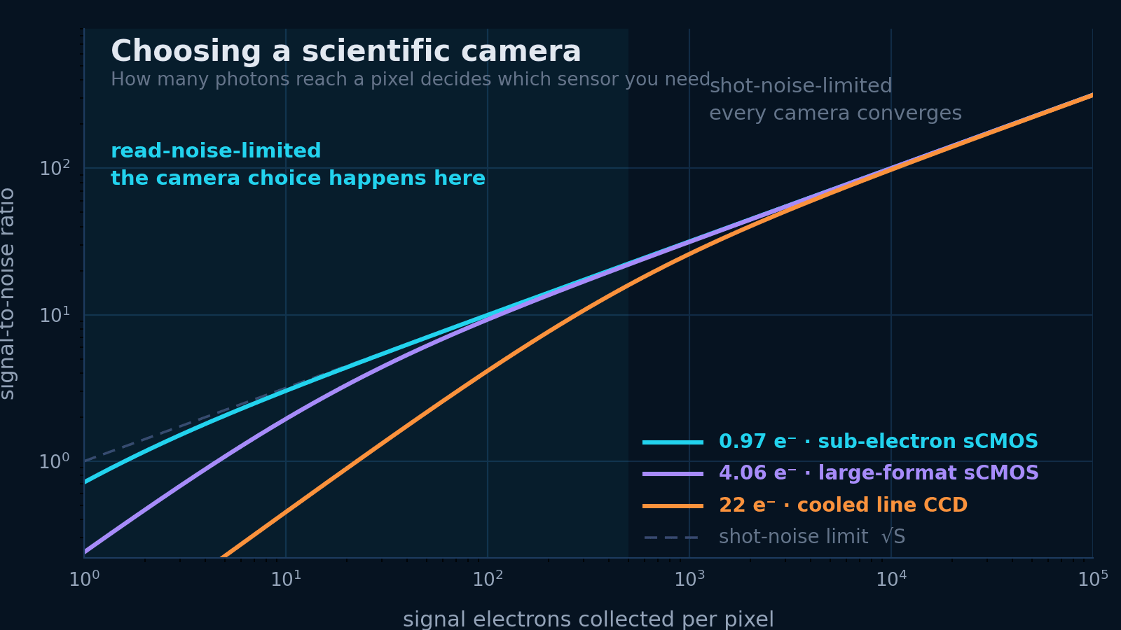
Read noise matters below the crossover and is irrelevant above it. Find which side you are on before comparing anything.
Timing decides the shutter
Rolling, global reset and global shutter answer different questions about what a single frame means.
Bandwidth decides the frame rate
A saturated interface silently throttles the camera. Pixels × bit depth × fps is a specification, not an afterthought.
The decision in one sentence
Count the photons first. Every other camera specification is downstream of that number.
Camera datasheets invite you to compare quantum efficiency against quantum efficiency and read noise against read noise. But whether a 0.97 e⁻ sensor beats a 22 e⁻ sensor by a factor of twenty or by nothing at all depends entirely on how much light arrives — and that is a property of your experiment, not of the camera.
Estimate the flux
Photons per pixel per frame, at the exposure you can actually afford to use.
Find the regime
Read-noise-limited, shot-noise-limited, or dark-current-limited. They have different answers.
Check the plumbing
Shutter mode, trigger behaviour and interface bandwidth — the specs that silently cap everything else.
1 · Noise regimes
There are only three ways to be noise-limited.
Read-noise-limited
Few photons per pixel, short exposure. The readout electronics contribute more uncertainty than the light does. A sub-electron back-illuminated sCMOS is worth real money here — and nothing else is.
Shot-noise-limited
Plenty of signal. Noise is √S, set by physics, and identical for every camera. The argument moves to full well, dynamic range, format, frame rate and sampling.
Dark-current-limited
Long exposures or infrared sensors. Thermally generated electrons accumulate with time, so the fix is cooling — not a quieter amplifier or a faster interface.
The whole model
Because read noise enters as Nr², it stops mattering quickly: it dominates only while S is smaller than Nr². At 1 e⁻ read noise that crossover is about one photoelectron. At 22 e⁻ it is nearly five hundred. That single fact explains most of the sCMOS-versus-CCD argument.
One camera has many read-noise figures.
On the sMAX04BM the same sensor reads out at 0.97 e⁻ in HDR 11HL, 1.72 e⁻ in 12-bit high-gain, 2.08 e⁻ with global reset, and 23.25 e⁻ in 12-bit low-gain — a twentyfold range that buys full well and speed in return. A read-noise number without its readout mode is not a specification, and comparing two cameras’ best-case modes tells you very little about how they behave in the mode you will actually use.
2 · Sensor technology
Six technologies, and only a few genuine decision points between them.
Wavelength rules out most of the list immediately. Photon flux settles most of the rest. What remains is usually a choice between format, speed and cost.
Back-illuminated sCMOS
- Signature
- Sub-electron read noise, 95% peak QE, megapixel formats at high frame rate
- Best for
- The default for scientific imaging: fluorescence, single-molecule, live-cell, quantitative microscopy, most spectroscopy
Watch: Rolling shutter by default, and per-pixel noise variation means the noise figure is a distribution, not a single number.
Front-illuminated sCMOS
- Signature
- Peak QE nearer 60–75%, otherwise the same architecture and speed
- Best for
- Signal-rich imaging where the extra QE does not change the answer and cost or NIR response matters more
Watch: At low light the QE gap compounds with read noise — the difference is larger in practice than the spec sheet suggests.
Deep-cooled CCD
- Signature
- Very large full well, uniform response, higher read noise, slow readout
- Best for
- Long-exposure spectroscopy and photometry where dynamic range per exposure beats frame rate
Watch: Read noise of tens of electrons is irrelevant at high signal and fatal at low signal. Readout is serial, so speed scales badly with format.
EMCCD
- Signature
- On-chip gain that makes read noise negligible, at the cost of an excess-noise factor of √2
- Best for
- Genuinely photon-starved work: single-photon counting, very low flux at high frame rate
Watch: Modern sub-electron sCMOS has taken most of the ground EMCCD used to own. The gain register also ages, needs recalibration, and throws away half your effective QE through excess noise.
InGaAs / SWIR
- Signature
- Sensitivity from roughly 900 to 1700 nm, where silicon is blind
- Best for
- NIR-II imaging, 1064 nm and telecom wavelengths, through-silicon inspection, moisture and hydrocarbon bands
Watch: Higher dark current, coarser pixels and smaller formats than silicon. Cooling is not optional at long exposure.
Industrial CMOS
- Signature
- High frame rate, small pixels, global shutter common, low cost
- Best for
- Alignment cameras, beam profiling, machine vision, anything where absolute photometry is not the point
Watch: Specifications are often typical rather than characterised, and there may be no defined QE curve or linearity guarantee at all.
Fast route
Four questions that eliminate most of the catalog.
Past 1 000 nm?
Yes → InGaAs. Silicon is not an option, whatever else it offers.
Under ~100 photons per pixel?
Yes → back-illuminated sCMOS, sub-electron mode.
Exposures over a second?
Yes → cooling is a specification, not an upgrade.
Is the frame one instant?
Yes → global shutter or global reset, and a real trigger input.
3 · Shutter + triggering
Decide what a single frame is supposed to mean.
A rolling-shutter frame is not a moment — it is a sequence of moments stacked into one image. That is invisible on a static sample under steady illumination, and it is the first thing that breaks when you add a pulsed laser or a moving stage.
Rolling shutter
Rows are exposed and read sequentially, so the top of the frame starts before the bottom
Lowest read noise and the highest frame rate an sCMOS can deliver — the reason it is the default mode
Moving objects skew, and a light pulse shorter than the frame illuminates only part of the sensor.
Global reset
All rows start together, then read out sequentially, so exposure length varies down the frame
Every row sees the same start instant, which is what a pulsed source or a single flash actually needs
Rows have different exposure durations, so a steady background is recorded as a gradient and has to be corrected.
Global shutter
All pixels start and stop together, holding charge until readout
Unambiguous timing: correct for fast motion, pulsed illumination and any frame that has to be one instant
Usually costs read noise, full well, or fill factor relative to the same sensor in rolling mode.
Pulsed illumination is the classic failure
Fire a laser pulse shorter than a frame period into a rolling-shutter camera and only the rows that happened to be integrating record it. The image shows a band, not a field. Global reset fixes exactly this: every row opens on the same trigger, so the pulse lands on all of them.
Specify the trigger, not just the shutter
Ask for trigger-in to exposure-start latency and its jitter, whether an opto-isolated input is provided, whether an exposure-active output exists for synchronising other hardware, and what happens to triggers that arrive during readout. A camera that accepts a trigger is not the same as a camera that is deterministic about it.
4 · Interface + bandwidth
The frame rate on the datasheet assumes the data can get out.
Pixels × bytes per pixel × frames per second is a hard number, and it is frequently larger than the interface a camera ships with. When it is, nothing errors — the camera simply runs slower than the number you bought it for.
GigE Vision
≈ 110 MB/s
Padded
100 m of standard cable, one connector, no grabber
Long runs and modest data rates
USB 3.0
≈ 350 MB/s
Padded
No frame grabber; ~3–5 m cable, host controller dependent
Benchtop cameras and most lab acquisition
Camera Link Base
≈ 255 MB/s
Packed
Frame grabber, deterministic timing and trigger latency
Synchronised acquisition at moderate rate
Camera Link Full / Deca
≈ 680 / 850 MB/s
Packed
Frame grabber, two cables, deterministic timing
High-rate line-scan and fast sCMOS
CoaXPress CXP-6
≈ 625 MB/s per lane
Packed
Coax; power, trigger and data on one cable, up to ~40 m
Long-cable high-rate acquisition
10GigE
≈ 1 100 MB/s
Padded
Standard networking hardware, needs a capable NIC and host
Large-format cameras at speed
Bit depth costs bytes — but how many depends on the interface
Camera Link and CoaXPress carry pixel taps at their native depth, so 12-bit costs 1.5 bytes. USB3, GigE and 10GigE pad to two bytes, so the same 12-bit camera generates a third more data on USB3 than on Camera Link.
ROI is the cheapest fix
Halving each dimension quarters the data. Most sCMOS also read a reduced ROI faster, so the frame rate rises at the same time.
The host is part of the path
Sustained writing to disk, PCIe lanes for the grabber, and CPU for any on-the-fly processing all sit between the sensor and your data.
5 · Regime lab
See which noise term owns your measurement.
Set the photon flux, exposure and detector, and the lab breaks the noise budget into its four terms, names the one that dominates, and tells you what a quieter sensor would actually buy. Then it checks whether your chosen interface can carry the frames at all.
Find your regime
Camera regime lab
Dim, fast, and dose-limited: read noise is usually what you are fighting.
Noise budget per pixel
total 8.33 e⁻ rms
The budget is now dominated by signal shot noise — the physical limit, which no camera can beat. That is a result of the 0.97 e⁻ readout, not of a generous photon budget: the same scene on a 23.3 e⁻ detector would give SNR 2.3 instead of 6.8, needing 8.8× the exposure to catch up.
4.19 MP at 12-bit and 108 fps is 679 MB/s against roughly 850 MB/s sustained. That leaves about 1.3× headroom for larger ROIs or deeper bit depth.
SNR = QE·S / √(QE·S + QE·B + D·t + Nr²), the standard photon-transfer model with independent noise terms added in quadrature. Read noise and QE are datasheet values for the selected model and readout mode; interface figures are practical sustained throughput for the standard, not marketing peak rates, and a real system also loses margin to the host, the cable and the grabber. Averaging N frames improves SNR by √N, which is why doubling it costs four times the acquisition time.
6 · Selection workflow
Six questions, in this order.
Answered in sequence, these eliminate whole categories before you compare a single datasheet — and they are the same questions we would ask on a specification call.
Photons per pixel per frame
Estimate it from source power, collection efficiency and exposure. Everything downstream is a consequence of this number — and it is the number most specifications are compared without.
Noise regime
Below the crossover, read noise and QE decide the result. Above it, shot noise does and the argument moves to full well, format and speed.
Wavelength
Silicon ends near 1100 nm. If any part of the signal is beyond it, sensor material is settled before any other specification is discussed.
Timing
Is the frame an instant or an interval? Pulsed illumination, moving samples and synchronised experiments constrain shutter mode and trigger behaviour.
Sampling
Pixel size, magnification and NA decide whether the optical resolution survives to the sensor. Fine pixels are not free — they divide the same photons further.
Data path
Pixels × bit depth × frame rate against a real sustained interface rate, plus the host that has to store it.
7 · Cameras
Back-illuminated sCMOS covers most of the decision space.
Sub-electron read noise, 95% peak quantum efficiency and megapixel formats at high frame rate is the combination that made sCMOS the default scientific detector. The exceptions — very deep wells, or wavelengths past silicon — are below it.
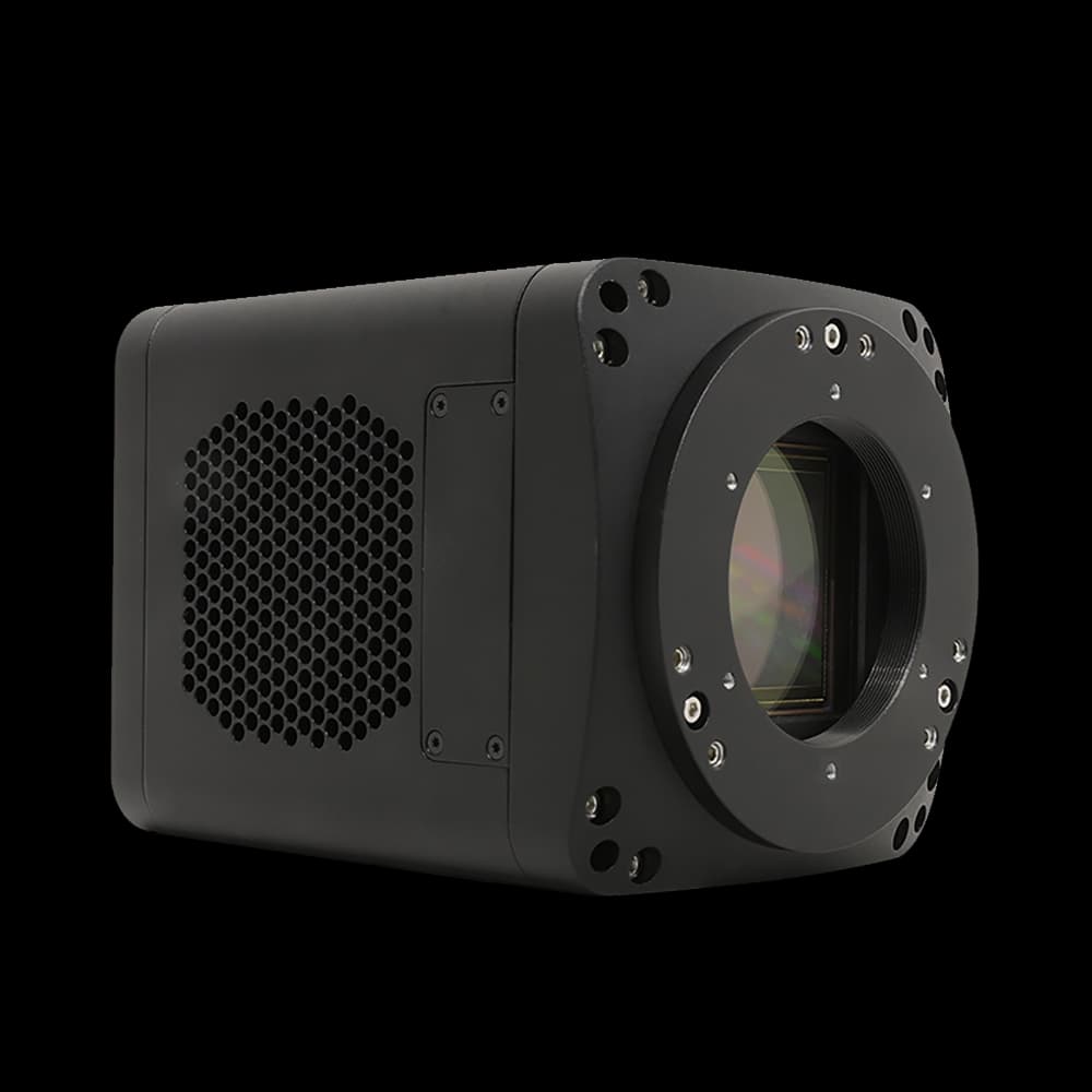
sMAX04BM-CL100
The 4.2 MP back-illuminated GSENSE2020BSI running at 108 fps full-frame over Camera Link, with 0.97 e⁻ read noise in HDR 11HL mode and rolling/global-reset readout. When an experiment is read-noise-limited and synchronised to something, this is the combination that matters.
- 0.97 e⁻ read noise (HDR 11HL)
- 95% peak QE @ 560 nm
- 108 fps @ 2048 × 2048
- Rolling shutter / global reset
- Camera Link · opto-isolated I/O
sMAX04BM-U100
The USB 3.0 variant of the same GSENSE2020BSI platform at 89 fps full-frame — the practical choice when the acquisition PC should stay simple and the timing budget allows a non-deterministic interface.
- Identical sensor and noise modes
- 89 fps @ 2048 × 2048
- 100 fps @ 1024 × 1024
- USB 3.0, no grabber required
- 12 µs – 10 s exposure range
sMAX16BM-U3-CL
A 16.8 MP GSENSE4040BSI on a 36.9 mm square sensor: four times the field of the 04-series at 90% peak QE, for whole-sample imaging where you would otherwise be tiling.
- 4096 × 4096 · 9 µm pixels
- 36.9 mm × 36.9 mm sensor
- 90% peak QE @ 550 nm
- USB3 and Camera Link on one body
- Up to 23 fps full frame
When sCMOS is not the answer
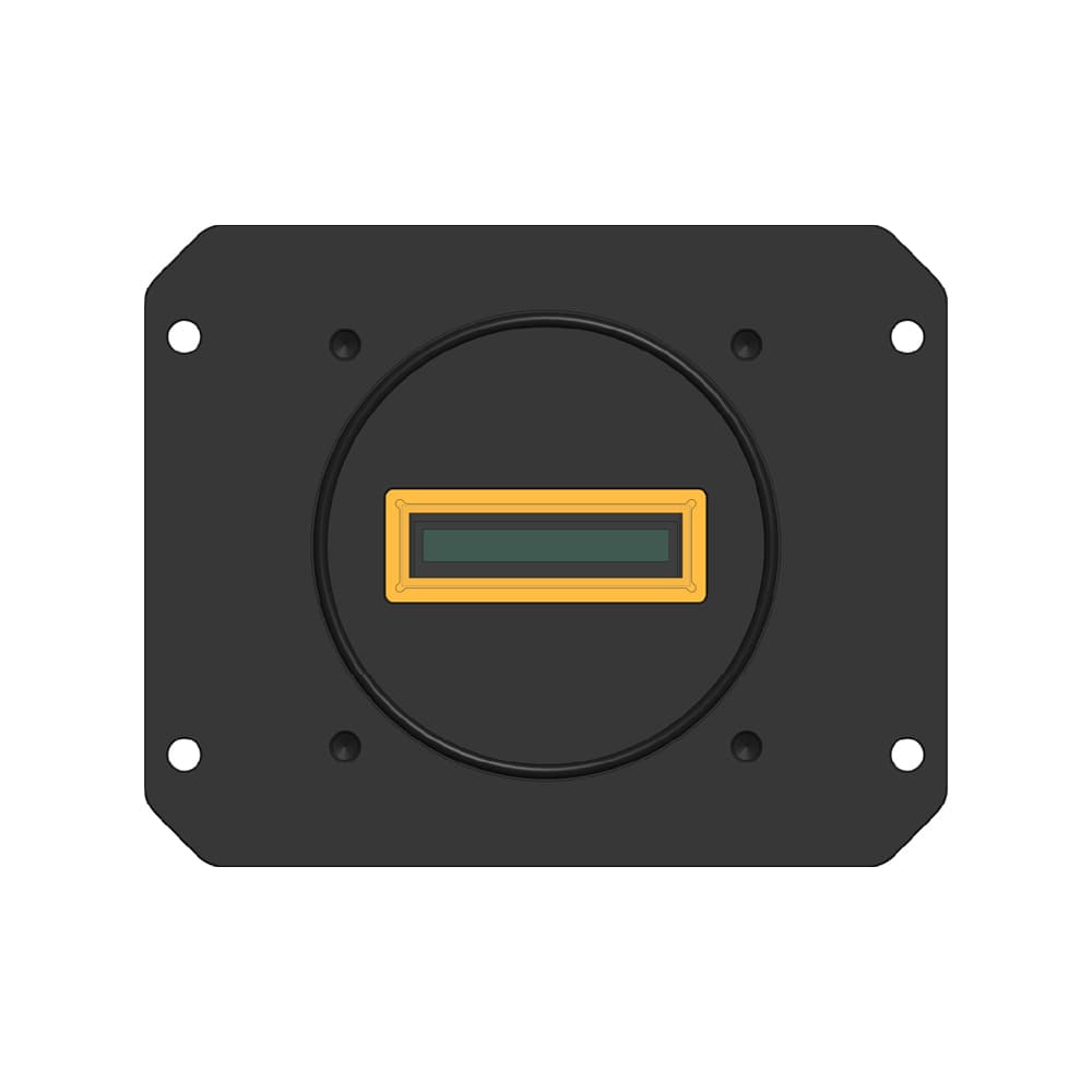
sCCD01AM
A deep-cooled 2048 × 1 E2V CCD261 with 459 ke⁻ full well and 95% QE at 800 nm. Read noise of 22 e⁻ is irrelevant at spectroscopic signal levels — what matters here is well depth, cooling and a 30.7 mm active length that matches a spectrograph focal plane.
- Sensor
- E2V CCD261
- Resolution
- 2048 × 1
- Pixel Size
- 15 µm × 15 µm
- Frame Rate
- 12 fps @ 2048 × 1
- Interface
- USB3
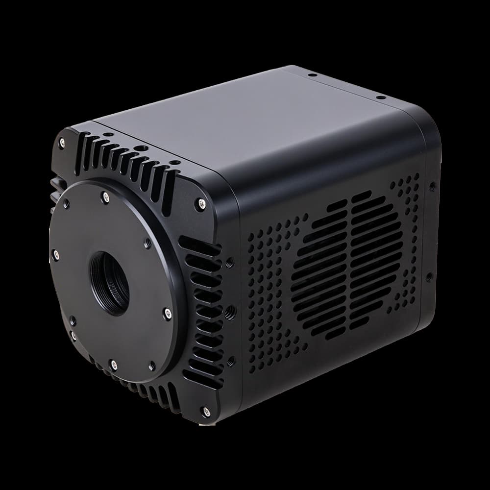
sNIRII640B-U3
A 640 × 512 InGaAs global-shutter camera with 15 µm pixels for NIR-II in-vivo imaging and anything past 1000 nm, where a silicon sensor records nothing at all regardless of its read noise.
- Sensor
- China-made InGaAs image sensor
- Resolution
- 0.33 MP (640×512)
- Pixel Size
- 15 µm × 15 µm
- Frame Rate
- Available on request
- Interface
- USB 3.0
Not sure which regime you are in?
Tell us the source, the optics between it and the sensor, the exposure you can afford and the field of view you need — that is enough to work out the photon budget and narrow the list to two or three cameras.
8 · Go deeper
Once the technology is settled, three guides finish the specification.
How to select an sCMOS camera
QE, read-noise modes, pixel size and SNR compared across real sMAX and MAX specifications, with a two-camera comparison lab.
Open guide Past the silicon cutoffWhen silicon isn't enough: choosing a SWIR camera
Why silicon stops at 1100 nm, what InGaAs sensor families offer beyond it, and how dark current and cooling drive the choice.
Open guide Sampling and opticsCamera field of view and diffraction sampling
Object-space pixel size, field of view and Rayleigh resolution — whether your pixels actually sample the optical resolution.
Open guide9 · Common questions
Short answers before the specification call.
Which camera technology should I choose?+
Start from how many photons reach a pixel in one frame. Below roughly a hundred photons per pixel you are read-noise-limited and a back-illuminated sCMOS with sub-electron readout gives the largest real improvement. Above it you are shot-noise-limited, every low-noise sensor performs about the same, and the decision moves to full well, sensor format, frame rate and cooling. If any part of your signal is past 1100 nm, the choice is made for you: InGaAs.
Is sCMOS better than CCD?+
For most scientific imaging, yes — modern back-illuminated sCMOS matches CCD quantum efficiency while offering far lower read noise and much faster readout. CCD still wins where a very large full well per pixel and highly uniform response matter more than speed, which in practice means long-exposure spectroscopy and photometry. A CCD read noise of 20 e⁻ is a non-issue on a spectrum of 100 000 electrons and a disaster on a 20-photon image.
Do I still need an EMCCD?+
Rarely. Electron multiplication makes read noise negligible, but the multiplication process adds an excess-noise factor of about √2, which is equivalent to halving quantum efficiency. Once sCMOS read noise dropped below about 1 e⁻, sCMOS matched or beat EMCCD for almost everything except genuine single-photon counting at high frame rate. The gain register also ages and needs periodic recalibration.
Rolling or global shutter?+
Rolling shutter gives the lowest read noise and highest frame rate, and is fine whenever the scene and the illumination are steady over a frame. You need global shutter — or at least global reset — when the sample moves quickly, when illumination is pulsed, or when the frame has to represent one instant. Global reset is the useful middle ground for pulsed sources: every row starts together, at the cost of a row-dependent exposure length you correct for.
How do I know the interface is fast enough?+
Multiply active pixels by bytes per pixel by frame rate. A 2048 × 2048 sensor at 12-bit and 108 fps is about 680 MB/s over Camera Link, which exceeds USB 3.0 and GigE by a wide margin. How many bytes a pixel costs depends on the interface: Camera Link and CoaXPress carry taps at their native depth, while USB3, GigE and 10GigE pad anything above 8-bit up to two bytes. A camera whose interface is saturated does not fail — it silently runs at a lower frame rate than the datasheet promises.
When does cooling actually matter?+
When dark electrons are comparable with your other noise terms — in practice, exposures beyond roughly a second, or any InGaAs sensor. Dark current roughly halves for every 5–7 °C of cooling, so deep cooling changes that term by orders of magnitude. For millisecond exposures it changes essentially nothing, and paying for it buys you a heavier camera and a fan.
Are these specifications comparable between manufacturers?+
Only if they are measured the same way. EMVA 1288 defines how QE, read noise, dark current, linearity and dynamic range should be characterised, and figures quoted against it can be compared directly. Numbers quoted as "typical" without a standard, or read noise quoted only in its most favourable readout mode, cannot. Always ask which mode a read-noise figure belongs to — on the same sensor it can vary by more than twentyfold.
How these numbers are measured
Quantum efficiency, read noise, dark current, linearity and dynamic range are only comparable between cameras when they are characterised the same way. The EMVA 1288 standard defines that method, and a figure quoted against it can be compared directly with another. When asking for specifications, three questions are worth more than any datasheet: which readout mode does this read-noise figure belong to, at what sensor temperature is this dark current, and is the quantum efficiency absolute or normalised?