How to Design a Fluorescence Spectrometer
Source, filters, sample geometry, monochromator, and detector as one coupled photon path. Translate fluorophore photophysics, Stokes shift, and sample state into a defensible optical architecture with an end-to-end photon budget.
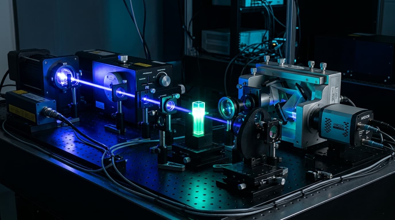 90° Cuvette · Czerny-Turner · sCMOS/PMT
The Coupled Optical Architecture
A fluorescence spectrometer is not an arbitrary assembly of isolated components. It is an end-to-end optical throughput and photon management system where every stage—from source spectral irradiance and excitation stray light rejection to sample collection geometry, dispersion efficiency, and detector read noise—must be quantitatively balanced against the fluorophore's transition physics.
Excitation Chain
Source spectral irradiance (P_exc), arc stability, clean-up filtering, and single vs. double monochromator stray-light rejection (10⁻⁵ vs. 10⁻¹⁰).
Sample & Geometry
90° right-angle vs. front-face (22.5°/30°), cuvette absorbance limits (A < 0.05), refractive index matching, and numerical aperture collection solid angle (Ω).
Emission Dispersion
Longpass edge blocking (OD ≥ 6), order-sorting filters, focal length (f), groove density (N), blaze wavelength (λ_B), and slit width (w).
Detection Chain
Point detector PMT (zero read noise in photon counting) vs. array sCMOS/CCD/InGaAs, quantum efficiency QE(λ), dark counts, and total SNR budgeting.
What a Fluorescence Spectrometer Measures
Photoluminescence occurs when a molecule absorbs a photon of energy hν_exc, promoting an electron from the singlet ground state (S₀) to an excited singlet state (S₁ or S₂). Following rapid non-radiative internal conversion and vibrational relaxation to the lowest vibrational level of S₁ within 10⁻¹² s (Kasha's rule), the fluorophore radiatively decays back to a vibrational level of S₀ on a nanosecond timescale (10⁻⁹ to 10⁻⁸ s), emitting a red-shifted photon hν_em.
The emission monochromator is locked to the peak emission wavelength (λ_em) while the excitation monochromator scans across the absorption band (λ_exc). The resulting trace reproduces the absorption spectrum of the fluorescent species, provided source intensity fluctuations are corrected with a reference detector.
The sample is excited at a single, fixed wavelength (λ_exc) while the emission monochromator or array spectrograph records the spectral intensity distribution across λ_em. Because emission occurs from the lowest vibrational level of S₁, the shape of the emission spectrum is strictly independent of excitation wavelength.
A 3D topographical landscape acquired by stepping λ_exc through a broad band and capturing complete emission spectra at every step. EEMs provide a comprehensive fingerprint for complex multi-fluorophore mixtures (e.g., dissolved organic matter in water, petroleums, proteins).
Steady-state spectrometers illuminate the sample continuously (CW) and measure time-averaged emission intensity. Time-resolved fluorescence (such as Time-Correlated Single-Photon Counting, TCSPC, or frequency-domain phase modulation) requires pulsed picosecond/femtosecond sources, fast PMTs or Hybrid Photodetectors (HPDs) with <50 ps instrument response functions (IRF), and high-speed timing electronics. This guide focuses on steady-state architecture.
Start with the Measurement: Translating Photophysics to Hardware
Instrument design must start from the physical properties of the target fluorophore and sample matrix, not from a catalog component list. The critical parameters that dictate hardware selection are:
| Photophysical Parameter | Physical Phenomenon | Direct Hardware Consequence |
|---|---|---|
| Stokes Shift (Δλ) | Δλ = λ_em - λ_exc. Energy loss during vibrational relaxation in the excited state. | Dictates filter edge steepness and stray light rejection. Shifts <20 nm require OD ≥ 8 ultra-steep edge filters or double monochromators to block Rayleigh scatter. |
| Molar Absorptivity (ε) & Quantum Yield (Φ_F) | ε (10,000–250,000 M⁻¹cm⁻¹) determines photon absorption rate; Φ_F (0.01–0.99) is emitted photons per absorbed photon. | Their product (ε × Φ_F) defines fluorophore brightness. Low brightness demands high f/# collection throughput and low-noise PMT/sCMOS detectors. |
| Sample Optical Density (A) | Absorbance A = ε · c · l. High concentration creates primary and secondary inner-filter effects (IFE). | For A > 0.1, right-angle 90° collection fails due to beam extinction before the cuvette center. Front-face (22.5°/30°) geometry must be used. |
| Spectral Line Width (FWHM) | Broad solution dye bands (30–60 nm FWHM) vs. narrow vibronic lines in aromatics / lanthanides (<0.5 nm FWHM). | Broad bands permit high-throughput, short focal length spectrographs (f=200 mm, f/3.5); narrow lines mandate high-dispersion f=500–750 mm systems. |
| Wavelength Regime | UV (200–400 nm), Visible (400–750 nm), NIR (750–1000 nm), SWIR (1000–1700 nm). | UV requires synthetic fused silica optics; visible uses silicon sCMOS / GaAsP PMTs; SWIR requires TE-cooled InGaAs detectors due to silicon's 1100 nm cutoff. |
Choosing the Excitation Source
The excitation source provides the initial photon flux. The primary trade-offs are spectral continuous tunability vs. monochromatic brightness, thermal/arc stability, and photobleaching risk.
Continuous Xenon Short-Arc Lamp (150W – 450W)
Gold Standard for EEMsHigh-pressure xenon short-arc lamps emit a smooth, high-color-temperature (~6000 K) continuum from 240 nm to over 1000 nm, interrupted only by sharp xenon emission lines between 800 and 1000 nm.
- Unrestricted Tunability: When paired with an excitation monochromator, allows scanning any arbitrary excitation wavelength.
- Arc Wander & Flicker: Convective cathode arc wander causes 1–3% high-frequency intensity fluctuations. Requires an internal reference photodiode channel to calculate S/R ratioed spectra.
- Ozone Safety: Lamps producing <240 nm output generate toxic ozone (O₃) unless ozone-free doped fused quartz envelopes or dedicated housing exhaust ducting are used.
High-Power LEDs & Lasers
High Brightness & StabilitySolid-state sources provide orders of magnitude higher spectral irradiance at discrete wavelengths, completely eliminating arc flicker.
- LEDs: Ultra-stable (<0.1% drift), long operating lifetime (>20,000 hrs), no warm-up time. FWHM is 15–30 nm. Dedicated excitation clean-up filters are mandatory to cut off broad sub-bandgap LED tails.
- Lasers (CW Diode / DPSS): Diffraction-limited spatial coherence and high mW–W powers for microscope coupling or trace detection.
- Photobleaching & Saturation: High laser power density (>100 W/cm²) rapidly destroys fluorophore populations via triplet-state photochemical pathways or causes ground-state optical depletion.
Excitation Wavelength Selection: Filters vs. Monochromators
The excitation selector isolates the desired wavelength band while rejecting out-of-band broadband source light by orders of magnitude.
Optical Bandpass Filter
Hard-sputtered dielectric interference filters deliver high peak transmission (>90%) with out-of-band blocking (OD ≥ 6). Compact and affordable, but restricts excitation to a single fixed wavelength band. Ideal for dedicated clinical or analytical instruments.
Single Monochromator
A Czerny-Turner monochromator (such as the Omni-λ200i or 300i) provides continuously motorized wavelength scanning. Typical stray light rejection is 10⁻⁵ (0.001%). Perfect for non-scattering, optically clear liquid solutions in standard cuvettes.
Double Monochromator
Couples two monochromator stages in tandem. Stray light rejection squares: (10⁻⁵)² = 10⁻¹⁰. Essential when exciting highly scattering matrices (biological tissue, liposomes, milk, solid powders) where diffuse excitation scatter would otherwise blind the emission detector.
Sample and Collection Geometry
The physical interface between excitation beam, sample volume, and emission collection optics determines what fraction of emitted photons enters the spectrograph and whether inner-filter artifacts corrupt the spectrum.
90° Right-Angle Cuvette vs. Front-Face Collection
Étendue & Numerical Aperture Matching
Optical throughput is governed by the conservation of étendue (G), defined as the product of the emitting area (A) and solid angle (Ω):
Light delivered faster than the spectrograph acceptance aperture (e.g., an f/1.5 lens focusing into an f/4.2 Omni-λ300i spectrograph) overfills the internal collimating mirror and diffraction grating. This overfilled light strikes mirror mounts, instrument walls, and grating edges, returning to the detector as diffuse stray light. Collection lenses must be chosen so their focal ratio matches the spectrograph f/#.
Emission Filtering: Optical Density & Edge Rejection
In typical fluorescence measurements, excitation photon flux exceeds fluorescence emission flux by 10⁵ to 10⁸ times. Without adequate emission filtering, Rayleigh and Mie scattered excitation photons swamp the emission signal.
Longpass edge filters transmit wavelengths longer than the cut-on wavelength while blocking shorter wavelengths. The optical density (OD = -log₁₀ T) at the excitation wavelength must satisfy:
For single-molecule or tight Stokes shift experiments, OD ≥ 8 (T ≤ 10⁻⁸) is mandatory.
Interference coatings shift to shorter wavelengths (blue shift) when light strikes at an angle of incidence θ or in a steep focusing cone:
In high numerical aperture microscope beams, steep cone angles broaden the filter edge and reduce out-of-band OD. Filters must be placed in collimated space.
Diffraction gratings obey m·λ = d·(sin α + sin β). Second-order diffraction (m=2) of UV excitation at 300 nm lands exactly at:
An order-sorting longpass filter (e.g. 400 nm cut-on) must be inserted before the emission spectrograph to eliminate phantom second-order peaks.
Monochromator and Spectrograph Selection: Equations & Trade-offs
The dispersion engine maps wavelengths onto the exit slit (monochromator mode) or across an array detector pixel plane (spectrograph mode). Czerny-Turner optical performance is governed by exact geometric diffraction relations.
1. The Grating Diffraction Equation
- • m: Diffraction order (typically m = 1).
- • λ: Wavelength in nanometers (nm).
- • d: Grating groove spacing in millimeters (d = 1 / N).
- • α, β: Incident and diffracted angles relative to grating normal.
2. Reciprocal Linear Dispersion & Bandpass
- • D⁻¹: Reciprocal linear dispersion in nm/mm.
- • N: Grating groove density in grooves/mm (e.g. 1200 g/mm).
- • f: Spectrograph focal length in millimeters (e.g. 320 mm).
- • w: Physical entrance slit width in millimeters (mm).
- • Δλ: Spectral bandpass (FWHM resolution limit).
Precisometer / Zolix Omni-λ Spectrograph Family Specifications
| Model | Focal Length & f/# | Dispersion (1200 g/mm) | PMT Resolution | CCD Resolution | Relative Throughput | Best Application |
|---|---|---|---|---|---|---|
| Omni-λ200i | 200 mm · f/3.5 | 3.58 nm/mm | 0.15 nm | 0.27 nm | 1.44× (Fastest) | High-throughput screening, broad dyes, LIF |
| Omni-λ300i | 320 mm · f/4.2 | 2.29 nm/mm | 0.08 nm | 0.173 nm | 1.00× (Reference) | General fluorescence research, photoluminescence |
| Omni-λ500i | 500 mm · f/6.5 | 1.49 nm/mm | 0.05 nm | 0.11 nm | 0.42× | Vibronic splitting, narrow organic lines |
| Omni-λ750i | 750 mm · f/9.7 | 1.02 nm/mm | 0.03 nm | 0.077 nm | 0.19× | Lanthanide emission, atomic lines, calibration |
| HiperS-320i | 320 mm · f/4.4 | 2.29 nm/mm | 0.06 nm | 0.12 nm | 0.91× | Multi-track fiber array, imaging spectroscopy |
Detector Selection: PMT, sCMOS, CCD, and InGaAs
The detector transduces dispersed photons into measurable electronic signals. Choosing between single-channel point detectors (PMTs) and multi-channel array detectors (sCMOS, CCD, InGaAs) fundamentally alters the signal-to-noise dynamics.
Photomultiplier Tube (PMT)
Point Detector (Scanning)PMTs use secondary electron emission across 8–12 dynode stages to provide noiseless internal electron gains of 10⁶ to 10⁷. In photon counting mode, discriminator thresholding eliminates electronic amplifier read noise entirely (σ_read = 0).
- • Bialkali (Sb-K-Cs): Peak QE ~30% in UV-blue (200–400 nm); ultra-low dark counts (<20 cps).
- • GaAsP Photocathode: Peak QE ~45% in visible (400–700 nm); sharp sensitivity cutoff past 720 nm.
- • Multialkali (S20): Extended red response up to 850 nm; higher dark current requiring TE cooling.
Back-Illuminated sCMOS & Deep-Cooled CCD
Array Detector (Spectrograph)Array detectors record all spectral channels simultaneously (multiplex/Fellgett advantage), enabling sub-second full spectral acquisition.
- • Back-Illuminated sCMOS: Peak QE >95%, sub-electron read noise (~1.0 e⁻ rms), megapixel resolution, no serial readout bottleneck.
- • Deep-Cooled Spectroscopy CCD (-70°C): Large full-well capacity (>100k e⁻), zero fixed-pattern column noise, lowest dark current for minutes-long integration times.
- • InGaAs Linear Array: Mandatory for SWIR photoluminescence (900–1700 nm). Requires -80°C multi-stage cooling.
The End-to-End Photon & SNR Budget
A quantitative photon budget calculates the survival probability of photons at each physical interface. Below is the full mathematical derivation from incident power to detected photoelectrons:
End-to-End Mathematical Derivation
σ_tot = √[ N_e + N_leak + N_auto + I_dark·t_int + σ_read² ]
Concrete Benchmark Calculation: Dilute Fluorescein (10 nM)
Consider a standard cuvette with 10 nM fluorescein (ε = 80,000 M⁻¹cm⁻¹, Φ_F = 0.90) excited with 1 mW at 488 nm (Φ_exc = 2.45 × 10¹⁵ photons/s) with f/3 collection (η_geom = 2.8%), T_optics = 40%, Δλ = 2 nm on a 35 nm broad band (f_bp = 5.7%), QE = 90% (sCMOS), and t_int = 100 ms:
Common Failure Modes & Engineering Mitigations
Even a perfectly specified spectrometer will produce invalid data if photophysical artifacts and optical aberrations are unaddressed.
When sample absorbance A > 0.1, the excitation beam is absorbed before reaching the center of the cuvette, reducing apparent emission intensity and distorting concentration calibration curves.
Fix: Dilute sample until A < 0.05 or switch to front-face geometry.
When the fluorophore has a small Stokes shift, emitted photons at the blue edge of the emission band are re-absorbed by unexcited fluorophores, artificially red-shifting the emission peak.
Fix: Reduce optical path length (1 mm cuvette) or front-face collection.
Water exhibits a prominent OH-stretching Raman band shifted by 3380 cm⁻¹ from excitation. At 350 nm excitation, water Raman appears at 397 nm, masquerading as a weak fluorescence peak.
Fix: Always record and subtract a pure solvent blank.
Diffraction gratings diffract light of wavelength λ in second order at the exact angle of 2λ. UV excitation at 280 nm appears as a false peak at 560 nm.
Fix: Insert an order-sorting longpass filter before the emission entrance slit.
Intense excitation photon density irreversibly destroys fluorophores. Furthermore, non-radiative relaxation increases with temperature (~1–2% loss per °C).
Fix: Attenuate excitation power, use sample shuttering, and utilize Peltier temperature-controlled cuvette holders.
PMT photon counters have dead times (~5–20 ns). High photon rates cause pulses to overlap, leading to severe non-linear undercounting.
Fix: Maintain count rates below 10⁶ counts/s or apply dead-time correction formulas.
Calibration, Standardization & Validation
Raw fluorescence spectra are distorted by wavelength-dependent grating efficiency curves, mirror reflectivities, and detector photocathode/sensor quantum efficiency. Traceable radiometric and wavelength calibration is required for publication and inter-laboratory comparability.
Relative Spectral Emission Correction
To obtain true emission spectra independent of instrument response, the system emission channel is calibrated using NIST Standard Reference Materials (SRMs):
- • NIST SRM 2940 (Mn-doped glass): Emission standard from 500 nm to 800 nm (excited at 412 nm).
- • NIST SRM 2941 (Uranyl-doped glass): Emission standard from 450 nm to 650 nm (excited at 427 nm).
- • NIST SRM 2942 (Ce-doped glass): UV emission standard from 320 nm to 430 nm (excited at 310 nm).
- • NIST SRM 2943 (Cu-doped glass): Emission standard from 350 nm to 640 nm (excited at 330 nm).
Wavelength Accuracy & Sensitivity Standards
- Wavelength Accuracy: Calibrated using low-pressure atomic emission pen lamps (Hg, Ar, Ne) with known atomic lines, or Holmium oxide solution (NIST SRM 2034) with sharp absorption bands.
- Water Raman SNR Benchmark: The universal standard for fluorescence spectrometer sensitivity. Measures the signal-to-noise ratio of the water Raman peak at 397 nm when excited at 350 nm with 5 nm excitation and emission bandpass:SNR_water = (I_Raman - I_background) / √(I_background)
Worked Engineering Examples
Compare how the complete hardware architecture shifts between two distinct spectroscopic regimes:
Broad Band, Large Stokes Shift (37 nm), Low Scattering
Target: Measure 10 nM fluorescein in buffer (λ_ex = 488 nm, λ_em = 525 nm, Φ_F = 0.90).
Tight Stokes Shift (20 nm), High Mie Scattering, Low Quantum Yield
Target: Measure trace carbon nanotubes / NIR dye (λ_ex = 785 nm, λ_em = 805 nm, Φ_F < 0.02) in scattering media.
Fluorescence Spectrometer Architecture Calculator
Input your fluorophore spectral bands, sample matrix, and resolution requirements to generate a complete, traceable optical hardware specification.
Quick Preset Scenarios
1. Measurement Parameters
High-Power Narrowband LED or Monochromatized Xenon Lamp
Cost-effective, highly stable (< 0.1% drift), long lifetime (> 20,000 hrs). FWHM is typically 15–25 nm, so a dedicated clean-up bandpass filter is required to remove LED spectral tails that would otherwise leak into the emission band.
Omni-λ300i (320 mm, f/4.2)
General research spectroscopy, balanced throughput & resolution
Back-Illuminated sCMOS or Deep-Cooled Spectroscopy CCD (e.g. 1024×256)
Broad dynamic range (> 16-bit), uniform pixel response, high quantum efficiency. Multi-track vertical pixel binning consolidates signal along the entrance slit height.
Geometry Best Practice: 90° Right-Angle Cuvette Collection
Standard for clear, dilute solutions (absorbance A < 0.05 at excitation peak).
- Use Suprasil synthetic fused quartz cuvettes to avoid intrinsic UV fluorescence from glass impurities.
- Couple collection with an f/2 or f/3 achromatic doublet or parabolic mirror matched to the spectrograph f/number.
- Keep sample optical density below 0.05 to avoid primary inner-filter attenuation of the excitation beam.
References & Authoritative Primary Sources
- Lakowicz, J. R. (2006). Principles of Fluorescence Spectroscopy, 3rd ed., Springer Science+Business Media, New York. DOI: 10.1007/978-0-387-46312-4.
- National Institute of Standards and Technology (NIST). Standard Reference Materials 2940, 2941, 2942, 2943: Relative Spectral Emission Correction Glass Standards. NIST Special Publication SP 260-153.
- Horiba Jobin Yvon / Instruments S.A. A Guide to Recording Fluorescence Spectra and The Optics of Spectroscopy Tutorial. Technical Monograph Series.
- Hamamatsu Photonics K.K. (2020). Photomultiplier Tubes: Basics and Applications, 4th ed., Electron Tube Division.
- IUPAC Recommendations (2011). Standards for Photoluminescence Quantum Yield and Emission Spectra Correction, Pure and Applied Chemistry, 83(12), pp. 2213–2228.
- National Institute of Standards and Technology (NIST). SRM 2034: Holmium Oxide Solution for Wavelength Calibration in the Ultraviolet and Visible Spectral Range.
FAQ
Frequently Asked Engineering Questions
Why is right-angle 90° collection standard in fluorescence spectroscopy?
In right-angle 90° geometry, collection optics are positioned perpendicular to the incident excitation beam. This geometric decoupling prevents intense direct transmitted excitation light from entering the emission monochromator, reducing stray light background by orders of magnitude compared to transmission spectroscopy.
When must I use front-face fluorescence instead of standard 90° cuvettes?
Front-face geometry (illuminating and collecting from the front cuvette window at 22.5° or 30°) is mandatory when sample absorbance exceeds A > 0.1, or when measuring turbid suspensions (liposomes, milk), opaque solid films, skin/tissue, or powders where excitation light cannot penetrate a standard 10 mm cuvette without severe primary inner-filter extinction.
What optical density (OD) is required for fluorescence emission filters?
Because excitation photon flux typically exceeds fluorescence emission flux by 10^5 to 10^8 times, emission filters must provide at least OD >= 6 (transmission <= 10^-6) at the excitation wavelength. For trace single-molecule measurements or small Stokes shifts (<20 nm), OD >= 7 to 8 is required.
How do I choose between a PMT and an sCMOS camera for fluorescence?
A Photomultiplier Tube (PMT) in single-photon counting mode provides zero readout noise, making it optimal for point-by-point wavelength scanning with a monochromator in low-light regimes. Back-illuminated sCMOS cameras provide >95% peak QE, ~1.0 e- rms read noise, and record the entire spectrum simultaneously across hundreds of pixels, making them ideal for rapid full-spectrum capture in spectrographs.
Why is second-order diffraction overlap a danger in fluorescence?
Diffraction gratings obey m*lambda = d*(sin alpha + sin beta). Second-order diffraction (m=2) of excitation light at wavelength lambda arrives at the exact physical angle of wavelength 2*lambda in first order. For example, 300 nm UV excitation appears as an apparent peak at 600 nm unless an order-sorting longpass filter is placed in the emission path.
Ready to configure your fluorescence spectroscopy system?
Tell us your excitation wavelength, target fluorophores, sample concentration, and required resolution. We will calculate the complete photon budget and verify grating turrets, filter sets, and detector matching.
Related Optical Guides
Explore companion spectroscopy & camera guides
Connect your fluorescence system design to spectrograph selection, scientific camera architectures, and optical filter specifications.
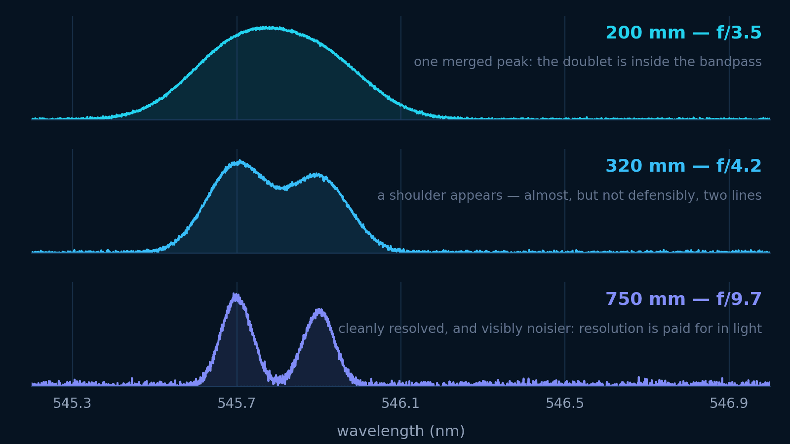 Spectroscopy
How to choose a spectrograph
Focal length, grating, and slit are one decision: how finely to spread the spectrum and how much light to pay for it. Watch a doublet merge and split through real Omni-λ dispersion numbers.
Open guide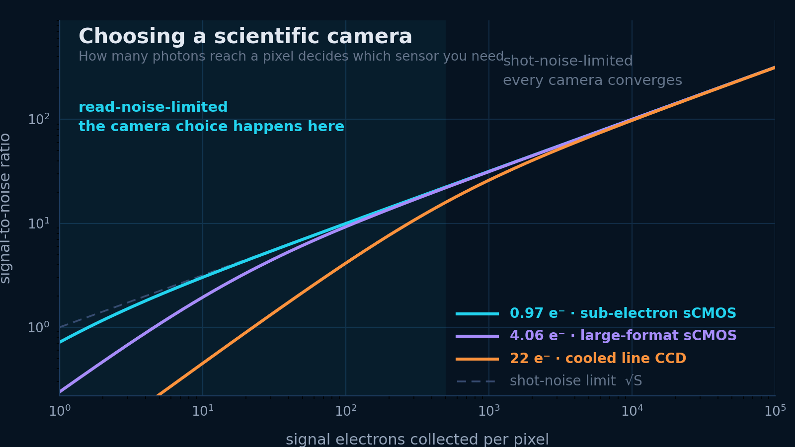 Scientific cameras
Choosing a scientific camera
Which sensor technology your photon budget actually needs, why rolling and global shutter answer different questions, and how to check the data can leave the camera at all.
Open guide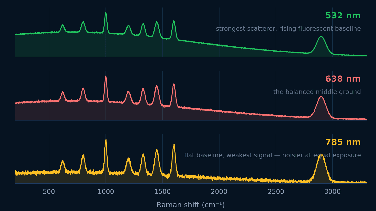 Raman spectroscopy
Choosing a Raman excitation wavelength
Balance the ν⁴ signal law, fluorescence background, silicon detector cutoff, and spatial resolution across 532, 638, and 785 nm.
Open guide