Recruit and relocalise
Pull a signalling protein to the membrane, the nucleus or an organelle in a chosen region, and watch what the rest of the cell does in response.
Cell biology · Application guide
You can project a two-micrometre pattern. Can you cause a two-micrometre perturbation?
Light-switchable dimerizers put protein recruitment, clustering and signalling under optical control. What limits the spatial precision is usually not the optics — it is how far the switched complex travels before it switches back.
01 / What patterned light controls
A light-switchable dimerizer couples one protein to another under illumination. Fuse one half to an anchor and the other to a protein of interest, and light becomes a way to relocalise, cluster or activate that protein — reversibly, and only where the pattern lands. A DMD pattern illuminator turns a drawn region into that pattern. [2][4][5]
Pull a signalling protein to the membrane, the nucleus or an organelle in a chosen region, and watch what the rest of the cell does in response.
Drive assembly of condensates or receptor clusters locally, then release the light and follow whether the structure persists.
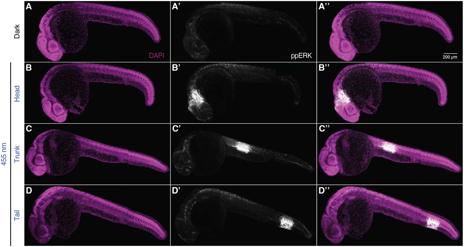
Hold different regions of an embryo or a culture under different light histories at the same time, in one field of view.
Jack et al. used an elliptical activation region to nucleate condensates at two telomeres in a living cell, bringing them together; when the light was removed the condensate shrank and the telomeres stayed merged. The experiment depends on activating a region smaller than the nucleus and on being able to stop. [6]
This is the regime where the distinction in this guide matters most. At this scale the projected pattern, the optical point-spread function and the molecular length scale are all comparable, and a claim about which structure was activated needs all three to be addressed.
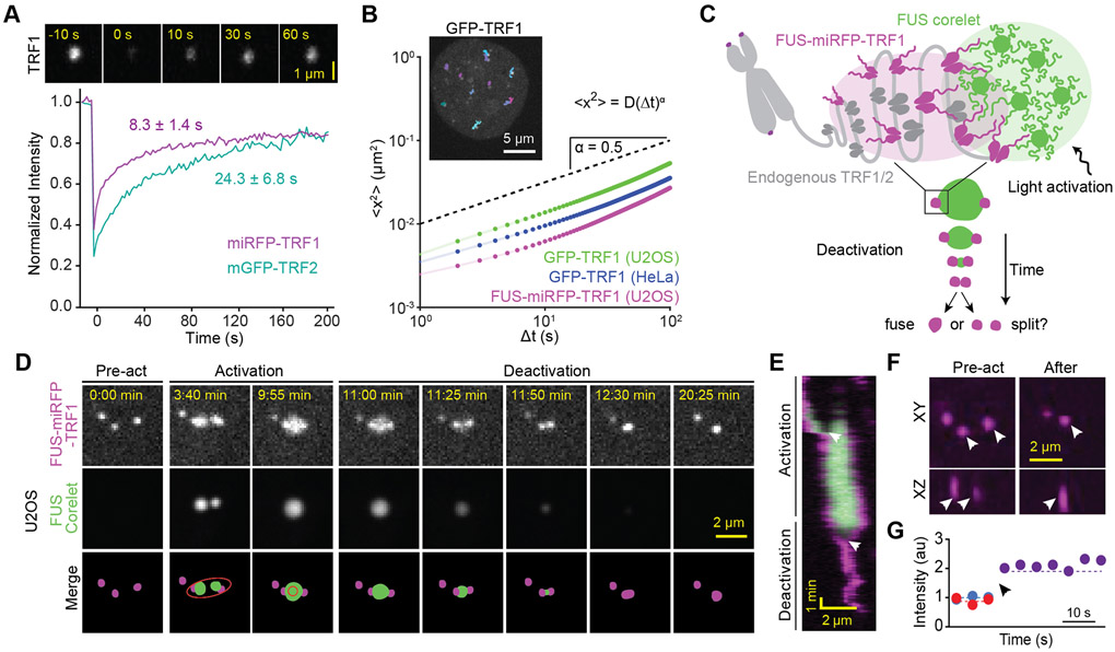
Published telomere measurements. Panels D and E show pre-activation, activation and deactivation; the ellipse in the merged schematic marks the local activation pattern.
Figure 1 from Compartmentalization of Telomeres through DNA-scaffolded Phase Separation. Amanda Jack, Yoonji Kim, Amy R. Strom, Daniel S. W. Lee, Byron Williams, Jeffrey M. Schaub, Elizabeth H. Kellogg, Ilya J. Finkelstein, Luke S. Ferro, Ahmet Yildiz and Clifford P. Brangwynne. Developmental Cell 57(2), 277–290 (2022). DOI. Reproduced under CC BY 4.0. Complete figure; no content changes. Display size and image encoding may differ. Accepted author manuscript deposited in PubMed Central; panel layout and resolution may differ from the version of record.
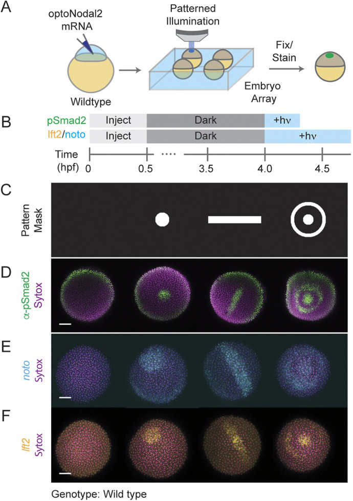
Published pattern masks (row C) and the resulting signalling and gene-expression patterns. A disc, a bar and an annulus produce matching patterns of pSmad2, noto and lft2.
Figure 2 from Optogenetic control of Nodal signaling patterns. Harold M. McNamara, Alison M. Guyer, Bill Z. Jia, Vicente J. Parot, Caleb D. Dobbs, Alexander F. Schier, Adam E. Cohen and Nathan D. Lord. Development 152(9), dev204506 (2025). © 2025. Published by The Company of Biologists. DOI. Reproduced under CC BY 4.0. Complete figure; no content changes. Display size and image encoding may differ.
At the other end of the scale, McNamara et al. patterned Nodal signalling across arrays of embryos, varying pattern geometry along one axis of the array and intensity along the other. Their reported projection path gives a 3.8 µm projected pixel at the sample, and they calibrate it by projecting a ten-spot mask onto a mirrored slide and fitting an affine transform from DMD to sample coordinates.[7]
Two details in their methods are worth copying rather than reinventing: they correct the illumination profile by imaging an all-on pattern reflected from a mirror and applying it as a grayscale correction, and they close an iris at the objective's back focal plane to make the projected pattern less sensitive to how the specimen sits relative to the focal plane.
02 / Where the precision actually goes
Once a complex forms on the membrane it diffuses. It keeps diffusing until it dissociates. Those two processes — a diffusion coefficient D and a lifetime τ — set a relaxation length λ = √(D·τ) over which the perturbation smears out, no matter how sharp the illumination was.[1]
Relaxation length
λ = √(D · τ)
For CRY2 recruited to membrane-anchored CIBN, Valon et al. measured D = 0.1 ± 0.03 µm²/s and a dissociation time of 185 ± 40 s. That gives λ ≈ 4.3 µm, and the authors report a practical spatial resolution of about 5 µm.
The published rendering of this equation drops the radical; the square-root form is what reproduces both the units and the authors' own figure.
The practical consequence is that below a few micrometres, shrinking the mask stops buying confinement and starts costing signal. The way out is molecular, not optical: shorten the lifetime outside the region. Levskaya et al. built exactly that into PhyB/PIF, illuminating the surroundings with far-red while driving the region with red, which they describe as using patterned light to defeat diffusive spreading. [1][3]
03 / Interactive spreading model
Assume a perfectly sharp projected edge, then add only diffusion and dissociation. The remaining spread is the part no optical improvement can remove.
Interactive / spreading model
Assume the projected edge is infinitely sharp. The recruited complex still spreads, because it diffuses in the membrane while it dissociates. Change the region and the molecular timing, and watch how much of the perturbation lands outside the light.
Diffusion and dissociation measured for CRY2 recruited to membrane-anchored CIBN. Valon et al. (2015)
Shortening the outside lifetime represents a second, antagonising wavelength that actively releases the complex everywhere except the region of interest.
Relaxation length
4.3 µm
√(D × lifetime) inside the region
Signal outside
39%
Share of bound complex beyond the mask
Peak reached
69%
Centre level vs whole-field illumination
Edge falloff
3.0 µm
To half the edge value, outside the mask
One-dimensional steady state of D·c″ − c/τ + S(x) = 0, with a uniform source inside the stripe and none outside. The solution relaxes over λ = √(D·τ) on each side. Concentration is plotted relative to the level whole-field illumination would reach.
Defaults are the values Valon et al. measured for CRY2 recruited to membrane-anchored CIBN: D = 0.1 µm²/s and a 185 s dissociation time, giving λ ≈ 4.3 µm, consistent with the ~4.5 µm the authors report. The antagonist preset uses the 4 s far-red release constant Levskaya et al. measured for PhyB/PIF.
Not modelled: optical blur, scattering, defocus and off-state background, all of which add to this spreading rather than replacing it; depletion of the cytosolic pool; CRY2 clustering and any cooperativity; photobleaching; three-dimensional and curved cell geometry; finite binding rates; transients before steady state. Percentages describe this model, not measured molecular specificity or a biological response. Measure confinement in your own preparation.
04 / Choosing the switch
Pick the light-switchable system first. It determines which colours you need, whether a second colour can turn it off, whether a chromophore must be supplied, and the lifetime that governs spreading. Properties below are as tabulated in the Krueger et al. review, with measured kinetics from the original tool papers. [5]
| System | Activation | How it switches off | Co-factor | Module size | What it is good for |
|---|---|---|---|---|---|
| CRY2 / CIB1 (CIBN) | 450 nm | Dark reversion, ~5 min | FAD — no exogenous chromophore | CRY2 57 kDa; CIBN 20 kDa | Recruitment and clustering. Translocation begins within ~300 ms of 488 nm illumination. CRY2 also oligomerises, which is useful for clustering experiments and a confound for pure recruitment.[2][5] |
| iLID (AsLOV2 / SspB) | 450 nm | Dark reversion, tunable by variant | FMN — no exogenous chromophore | AsLOV2 16 kDa; SspB 13 kDa | Heterodimerisation with a small tag and more than a 50-fold affinity change on illumination. Tunable off-kinetics let you trade confinement against the light dose needed to hold a gradient.[4][5] |
| PhyB / PIF6 | 660 nm on; 750 nm off | Light-driven at 750 nm; dark reversion ~20 h | Phycocyanobilin or phytochromobilin — must be supplied | PhyB ~100 kDa; PIF6 11.5 kDa | The only listed switch you can actively turn off with a second colour. Measured time constants of 1.3 ± 0.1 s to recruit and 4 ± 1 s to release. Red and far-red leave the blue–green spectrum free for imaging.[3][5] |
| Magnets (pMag / nMag) | 450 nm | Dark reversion, tunable seconds to hours | FAD — no exogenous chromophore | 16 kDa | Heterodimerisation with the widest published range of tunable kinetics, when the experiment needs a specific lifetime rather than the fastest one.[5] |
Dark-reversion times are the review's tabulated values and vary with variant, temperature and expression level. Measure the kinetics in your own preparation before relying on them for a confinement or dose calculation.
CRY2, iLID and Magnets all activate near 450 nm, which overlaps GFP excitation and most blue-excited indicators. Emission filters keep stimulation light out of the camera, but nothing in the detection path stops imaging light from driving the switch. Plan excitation dose, interleaving and reporter choice together with the switch.
PhyB/PIF moves activation to 660 nm and release to 750 nm, freeing the blue–green range for imaging and giving an active off-switch for the surroundings. The costs are a supplied chromophore, a large module, and a two-colour optical path — which is where a dual-input illuminator and beam combiners enter the configuration. [3][5]
05 / Configuration and equipment
Once the switch fixes the colours, the rest of the path follows: how light is coupled into the illuminator, how the pattern reaches the objective, how the port is shared with a camera, and how everything is triggered.
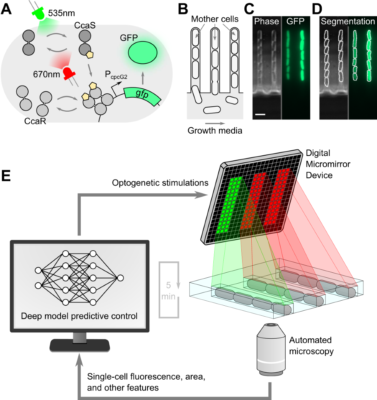
Published closed-loop platform. Panel E shows the control cycle: image the cells, segment them, compute a per-chamber pattern, and project it with the DMD before the next interval.
Figure 1 from Deep model predictive control of gene expression in thousands of single cells. Jean-Baptiste Lugagne, Caroline M. Blassick and Mary J. Dunlop. Nature Communications 15, 2148 (2024). © The Author(s) 2024. DOI. Reproduced under CC BY 4.0. Complete figure; no content changes. Display size and image encoding may differ.
Anderson et al. itemise their path: a Polygon 1000 fed by a Mightex collimated LED through two beam combiners in series, routed into a Zeiss LSM 800 through an infinity port expander, with the region of interest defined in PolyScan4 and a 10×/0.3 objective at the sample. They report a 170 × 170 µm square at 11.42 W/m² for one minute. [8]
One detail is worth pausing on. The authors describe the source as a 455 nm LED and cite part number BLS-LCS-0470-14-22, which the current catalogue lists as a 470 nm emitter. Whatever the explanation, it is a reminder to confirm the emitter and its measured spectrum against the switch's action spectrum rather than inheriting a wavelength from a methods section.
Closed-loop work adds a timing requirement rather than a different illuminator: Lugagne et al. recompute each chamber's pattern between frames, so pattern upload, source switching, exposure and analysis all have to fit inside the control interval. [9]
Decide in advance whether the experiment needs "this cell and not its neighbour", "this half of the cell", or simply "a graded perturbation". Each demands a different confinement budget, and only the first two force you to fight diffusion.
The switch fixes the activation wavelength, whether a second colour can turn it off, whether a chromophore must be supplied, and the lifetime that sets spreading. Changing it later changes the whole optical path.
List activation bands and every imaging band. Check that imaging light cannot drive the switch, as well as that stimulation light cannot reach the detector. Clean emission filters solve only one of those two problems.
Measure the projected edge on a calibration target, then measure the perturbation in the preparation. They are different widths, and improving the first does not fix the second.
Map camera to DMD coordinates with a known target, and measure the illumination profile across the field so the pattern delivers the dose you think it does. Repeat per objective and after any optical change.
Record power at the sample plane with a calibrated detector, together with objective, source setting and active mask area. Irradiance changes when ROI area changes; dose is irradiance times time.
Include unilluminated cells in the same dish, a no-switch control, and a region far from the ROI. A response in the surroundings may be diffusion, scattered light, or signalling — plan to distinguish them.
If the experiment is triggered or closed loop, measure optical onset against acquisition with a photodetector. Software timestamps do not establish when light reached the sample.
Mightex systems and components available through Precisometer, with part numbers, variant tables and configuration options. Where a published setup names a part, it is noted below — a starting point for a specification, not a guarantee that the configuration transfers to another microscope.
Dual input: lightguide + laser fibre
Accepts both a lightguide-coupled LED and a laser fibre, so two delivery formats reach one DMD. Verify each path separately.
Pattern illuminator (liquid lightguide)
Lightguide-coupled DMD illuminator spanning 350–1000 nm, the usual route for LED-driven blue and red switches.
Ultra-high contrast, laser fed
Worth assessing when residual off-state light, rather than diffusion, is what limits your dark regions. 400–700 nm.
Collimated LED sources, 22 mm aperture
The BLS-LCS collimated family from 365 to 980 nm plus white. Anderson et al. cite part number BLS-LCS-0470-14-22 from this family.
Merge two collimated sources
Dichroic combiners, cascadable for more wavelengths. Anderson et al. cite LCS-BC25-0435 and LCS-BC25-0515 in series.
LED into a liquid lightguide
High-efficiency coupling of LED output into a 3–8 mm liquid lightguide, the input format a Polygon1000-G expects.
Share one infinity port
Expands one infinity-path port into two to four, so a Polygon, a camera and a scanner can share it. Anderson et al. route the DMD through an IPX.
Calibration, ROI design, sequencing
Camera-to-DMD calibration and pattern sequences. Anderson et al. define their square ROI in PolyScan4. Confirm version, licence and camera support.
Infinity-port optical coupling
Stand-specific adapters for Nikon, Olympus, Leica and Zeiss uprights and inverteds.
Trigger and synchronisation
Event timing and multi-channel triggering where stimulation, imaging and perfusion have to agree on a clock.
Calibration targets and optics
Grid calibration slides, filter holders and alignment tools — the parts that make registration checkable.
Source gating and modulation
Drive and gate the LED source. Pattern switching on the DMD is separate from how fast the source itself turns on and off.
Related building blocks: filters and dichroics, scientific cameras, and laser sources where a laser-fed illuminator is appropriate. Confirm software version, licence tier and camera support before assuming an integration is supported.
06 / Controls and interpretation
In a patterned experiment the unilluminated area is not empty space — it is the control that carries the spatial claim. Decide in advance what a response there would mean, and how you would tell diffusion, stray light and genuine signalling apart.
| Symptom | Checks |
|---|---|
| The response extends well beyond the ROI | Separate the causes before changing the mask. Check off-state background and scattering optically; then compare the measured width against the relaxation length for your switch. If the length scale explains it, a smaller ROI will not help — a faster-reverting switch or an antagonist wavelength will. |
| Neighbouring cells respond too | Check registration and field flatness first, then whether the readout itself is diffusible or the pathway is non-cell-autonomous. Cell-to-cell signalling is not an optical problem and will not improve with a sharper edge. |
| Imaging activates the switch | Reduce excitation dose, shift the imaging fluorophore, interleave acquisition, or move to a red/far-red switch. A detection filter cannot prevent imaging light from driving a blue-light switch. |
| Signal fades during a long hold | Distinguish photobleaching of the reporter, depletion of the recruitable pool, adaptation, and loss of the switch to dark reversion. Record a no-stimulation photobleaching control in the same session. |
| The perturbation is confined but weak | A short complex lifetime sharpens the edge and lowers the plateau. Raising irradiance may restore amplitude, but check for heating and phototoxicity before treating power as free. |
Practical answers
Not by itself. The projected pattern sets where light arrives. The recruited complex then diffuses in the membrane while it dissociates, and that pair sets a relaxation length of roughly the square root of the diffusion coefficient times the lifetime. For CRY2/CIBN, Valon et al. measured about 4.5 µm. A smaller mask does not shrink that length; it only reduces how much signal you get. Optical blur and scattering add to this and are a separate budget.
Shorten the lifetime of the complex outside the region rather than shrinking the mask. A switch with a second, antagonising wavelength — PhyB/PIF with far-red — lets you hold the surroundings in the off state while the region is driven on, which Levskaya et al. describe as defeating diffusive spreading with patterned light. Faster-reverting variants of blue-light switches work in the same direction. Both cost amplitude: a faster reset means a lower steady-state level inside the region.
At least the activation band, plus every imaging band you intend to use. Blue switches overlap GFP and most blue-excited indicators, so imaging light can activate the switch even when the detection filters are clean. PhyB/PIF moves activation to 660 nm and release to 750 nm, which frees the blue–green range for imaging but requires an exogenous chromophore. Plan the activation and imaging spectra together, in both directions.
Treat it as a starting point, not a parts list. Anderson et al. itemise their LED, beam combiners, port expander and objective, which makes their configuration unusually reproducible — but the delivered irradiance, field and registration still depend on your stand, relay and objective. Confirm every part against current specifications, and measure power and registration at your own specimen plane.
Published work does exactly that: Lugagne et al. segment cells from each frame and compute a new per-chamber pattern within the imaging interval. It requires that pattern upload, source switching, camera exposure and analysis all fit inside your control period, with a shared timing reference. Measure that budget on the assembled system rather than assuming the DMD switching rate is the limit.
From experiment to configuration
The switch, the smallest region you need and the readout together determine the illuminator, the source, the microscope interface and the timing. Send those and we can assess a configuration.
Sources and image rights
The research figures on this page come from the articles named in their captions. All four are covered by Creative Commons Attribution 4.0, which permits commercial redistribution with attribution, a licence link and an indication of changes. Each caption was checked for a separate third-party credit; figures carrying one are not used here.
Keep each figure's attribution and licence notice when reusing it. Resizing and image encoding for web display do not change the scientific content. Reuse does not imply endorsement by the authors or publishers. The figure licences cover those figures only; other referenced papers retain their own terms.
Download the image attribution and licence record ↗Official Mightex brochures for the illuminators discussed above:
Optical inputs, wavelength ranges, field and projected-sampling tables, switching speeds and trigger timing.
Laser-fed input, 400–700 nm support, and the all-on / all-off definition behind its contrast figure.
Licences and manufacturer specifications verified October 2026. Polygon and PolyScan are Mightex products distributed by Precisometer. The interactive model is an illustrative calculation with the assumptions stated beside it, not a prediction of molecular specificity or a biological response. Configuration recommendations remain subject to the exact microscope, optical components, software and preparation.
Before you specify
Targeted stimulation and recording in neurons, image-guided spatial barcoding, and maskless photolithography.
 Optogenetics
Plan targeted illumination in neuronal cultures or tissue slices: compare Polygon inputs, register camera ROIs, verify delivered light, and synchronize electrophysiology or compatible imaging. Includes an interactive pattern illustration.
Open guide Spatial biology
Connect regions selected in a tissue image to molecular barcodes and sequencing. Explore the published Light-Seq application, a barcode-group lab, registration geometry and the Polygon optical setup.
Open guide Microfabrication
Follow a digital mask from mirrors to material. Explore four Polygon application workflows, compare single-photon and research two-photon architectures, and try the exposure and pulse-scaling labs.
Open guide