01
Draw
Create a bitmap, line pattern or region of interest. Its pixels define where light is requested.
A visual field guide
DMD maskless photolithography. How it works, what Polygon makes easier, and what changes when you move from one photon to two.
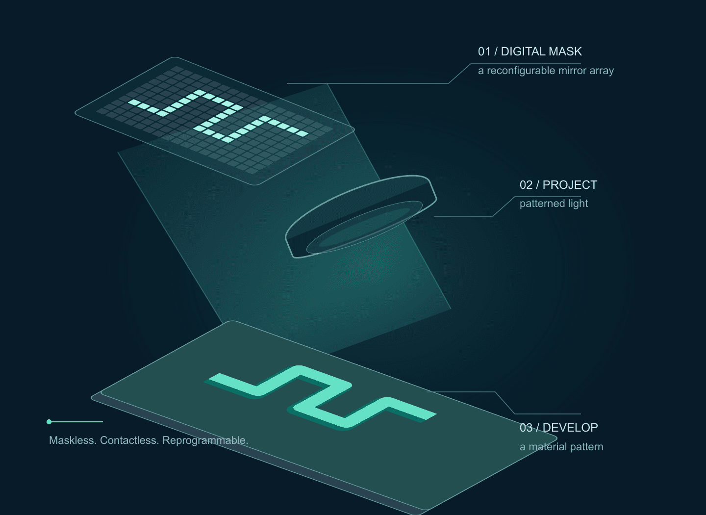
01 / The principle
A digital micromirror device replaces a physical photomask with an array of tilting mirrors. On mirrors send light into the projection optics; off mirrors send it away. Change the file and the next exposure can have a new shape.
01
Create a bitmap, line pattern or region of interest. Its pixels define where light is requested.
02
Image the DMD onto the work plane through a calibrated relay and objective.
03
A matched photoinitiator or photosensitive group changes the material where exposure is sufficient.
04
Develop a resist, wash away uncured precursor, or read out a patterned surface reaction.
Maskless exposure removes mask fabrication from the iteration loop. Coating, alignment, exposure calibration and material processing still determine the result. Polygon application context: [2][3]
02 / Choose the physical process
1P / linear absorption
One absorbed photon can initiate the chemistry. UV or visible light exposes a resist, hydrogel or functional surface. Optical focus alone does not provide intrinsic depth confinement.
2P / nonlinear absorption
Two photons contribute to one excitation through a nonlinear process. Reaction depends on intensity squared; a tightly focused, ultrashort pulse can confine polymerisation around a focal region.
| Design question | Single-photon projection | Two-photon lithography |
|---|---|---|
| What is written? | A surface pattern or exposed film; stacked layers with added z control. | Voxels, multiple foci, or a temporally focused patterned layer. |
| What sets the dimensions? | Projected sampling, optical contrast and material processing. | Focus geometry, pulse conditions, nonlinear threshold and chemistry. |
| Where is it useful? | Fast design iterations, hydrogel patterns, resist masters, surface chemistry. | 3D scaffolds, micro-optics and structures requiring internal depth control. |
| How does Polygon fit? | A packaged pattern projector and microscope integration route. | A standard Polygon is not documented as a turnkey two-photon writer. |
The 2P excitation spectrum must be measured or supplied for the initiator; doubling a one-photon wavelength does not establish a useful two-photon cross-section. The 3D mechanisms are demonstrated in [6][7][8]
03 / Single-photon exposure lab
Change the feature width, optics and exposure. Watch the same pattern pass from binary mirrors to delivered light to retained resist. Try a long exposure with residual light to see why dark regions matter.
Interactive / mask → light → material
Projected pixel
0.38 µm
Full field
495 × 310
µm · Nikon G, standard relay
Rayleigh reference
0.56 µm
0.61 λ / NA
On-field dose
100.0 mJ/cm²
Bright = mirror on
Bright = higher irradiance
Gold = remains; slate = removed
Same 36.5 × 24.3 µm crop in all three views. The crop uses 96 × 64 DMD pixels.
The intended regions cross threshold. Change dose to watch the edges move.
D = I × t, using mW/cm² and seconds to give mJ/cm². The threshold is an arbitrary user input, with the same ideal step response used for positive and negative tone.
The Nikon Polygon1000-G standard-relay values are 9.9 × 6.2 mm and 7.6 µm per pixel at 1×, divided by objective magnification. Other microscope relays and Polygon models need their own calibration. Magnification and NA are independently adjustable here.
The binary mask is sampled at DMD-pixel centres, expanded 3× for calculation, and convolved with a Gaussian intensity PSF, σ = 0.21 λ / NA. A uniform residual-light fraction is then added. This approximates incoherent projection; the Rayleigh distance is a point-separation reference, not a printed linewidth guarantee.
This is a thin-film, in-focus model. It omits coherent speckle, defocus, distortion, absorption, standing waves, bake chemistry, diffusion, oxygen inhibition, shrinkage and development kinetics. Residual-light settings are illustrative and are not Polygon contrast specifications.
A projected DMD pixel is a placement increment. A single-pixel line is not automatically a reliable printed line.
NA, wavelength, focus and aberrations determine contrast. Coherent laser illumination can add speckle and diffraction artefacts.
Exposure, film thickness, bake and development shift the final edge. Verify linewidth and gap clearing on a test coupon.
04 / Build with Polygon
Polygon packages the DMD, projection module and microscope coupling. PolyScan provides pattern design, sequences and calibration tools. This makes single-photon prototyping more approachable; the exposure process still needs development for your material. [1][4]
Choose a supported infinity-path adapter and objective instead of building a DMD relay from scratch.
Microscope adaptersCreate or import patterns, map image coordinates to projected coordinates, then run an exposure sequence.
PolyScan softwareSelect lightguide or laser-fibre coupling and verify delivered power, uniformity and wavelength transmission.
Light sources| Polygon model | Optical input / stated range | Lithography planning |
|---|---|---|
| Polygon1000-G | 3 mm liquid lightguide · 350–1000 nm | Candidate for 365 nm exposure with a suitable source and UV-transmitting downstream optics. |
| Polygon1000-DL | SMA laser fibre · 400–1000 nm | Candidate for 405 nm chemistry; 365 nm is outside its stated range. Circular projected field. |
| Polygon1000-DI | Lightguide: 350–1000 nm; fibre: 400–1000 nm | For 365 nm, assess the lightguide path. Confirm each input separately. |
| Polygon UHC | SMA laser fibre · 400–700 nm | Candidate for background-sensitive visible-light chemistry. 365 nm is outside its stated range. |
An SU-8 process is one possible starting point: the cited SU-8 2000 data recommends 365 nm and includes a post-exposure bake. Evaluate a G or DI lightguide configuration, UV optics, a calibration target and a dose matrix. Choose the exact formulation and process from its current supplier data. [5]
Use a precursor and initiator validated at 405 nm. Screen formulation, oxygen inhibition, substrate adhesion and wash conditions. Start with islands and line/gap coupons before a device layout; verify cell compatibility separately when relevant. Polygon microfluidic applications include hydrogel fabrication and curing. [3]
The brochure specifies up to 6,600 frames/s at 1-bit depth. A pattern refresh rate does not determine the time needed to expose a resist. Confirm grayscale timing, minimum stable source pulse and trigger behaviour for the chosen configuration. PolyScan camera support depends on the model and licence. [1][4]
For 1P exposure, temporal duty q gives D ≈ q × Ion × t when the source and material behave linearly over that timing range. For 2P excitation, pulsing the same peak illumination on for fraction q gives ⟨I²⟩ ∝ q × Ion²; it is not equivalent to reducing continuous intensity to q × Ion. Grayscale requires calibration.
UHC’s stated 10,000,000:1 ratio compares all-on and all-off images. It does not establish local dark-region contrast beside bright features in a resist. Measure background and edge leakage with the actual mask and exposure duration. [10]
05 / Applications
Polygon is worth evaluating when the experiment needs selected surface regions, changing illumination masks or a spatial exposure map. These examples show useful workflows; the advantages described here are engineering interpretations of the cited demonstrations.
Change the layout in software; illuminate multiple regions together.
Mightex reports patterned exposure of an acrylate film using Polygon and a 400 nm LED.
Before relying on it: Measure linewidth, film thickness and exposure uniformity.
Manufacturer-reported demonstration [2]
Select which membranes receive the intended exposure in a registered field.
A published Polygon400 study used photodegradable hydrogel membranes to retrieve bacteria from selected microwells.
Before relying on it: Validate registration, background exposure and retrieval in your preparation.
Published study · historical Polygon400 setup [12]
Revisit a field with different illumination masks during observation.
Mightex reports light-driven protein dissociation on a coverslip, followed by rebinding in the dark.
Before relying on it: Verify chemistry-specific reversibility and imaging compatibility.
Manufacturer-hosted laboratory demonstration [2]
Encode spatial differences in surface attachment through an exposure map.
A Polygon1000 application report describes 365 nm functionalisation of glass, with local exposure time used to vary attached dye density.
Before relying on it: Calibrate the dose-to-attachment response for the actual surface chemistry.
Researcher application report · manufacturer-hosted [13]
Original conceptual drawings; no measured response, exposure time or fabricated dimensions are represented.
A microscope-based Polygon workflow may suit surface photochemistry or selected-region exposure in an existing experiment. A dedicated two-photon fabrication system addresses additional requirements such as freeform 3D geometry and controlled writing in depth. Nanoscribe documents these capabilities for Quantum X shape. [14]
Hydrogels and custom materials are also supported by Nanoscribe Quantum X bio. Material flexibility alone does not establish a Polygon advantage. [15]
The sources above do not establish a head-to-head ranking. Compare the same target geometry and material for total processing time, reliable feature size, surface quality, alignment and yield before making a speed, cost or accuracy claim.
06 / Two-photon lithography
Published systems use a DMD for either holographic multi-focus writing or patterned-plane projection with temporal focusing. Both need ultrafast pulse delivery and suitable two-photon chemistry. They are distinct research architectures. [6][7][8]
Route A / multiple foci
A binary hologram redistributes the wavefront to selected foci. The hologram is not a direct image of the printed shape. Geng et al. demonstrated parallel, independently controlled writing with a custom DMD scanner. [7]
Route B / patterned plane
Spatial and temporal focusing bring the shortest pulse to the build plane. Saha et al. demonstrated patterned-layer fabrication with a DMD. Pulse recombination supplies depth selectivity that ordinary wide-field projection lacks. [6][8]
The cited Polygon documents establish patterned illumination, not a qualified femtosecond lithography path. A nominal 800 nm transmission range does not establish pulse preservation, dispersion compensation, diffraction-order collection or pulse-damage tolerance. Common 1030 nm sources also sit outside the G/DL/DI stated upper wavelength limit. A 2P design requires a dedicated optical review and manufacturer confirmation. [1][9]
This lab uses a point-focus model to show intensity-squared scaling. Double the number of foci at fixed total power and the drive per focus falls fourfold. Stretch the pulse and the nonlinear drive falls too.
Interactive / why peak intensity matters
Compare trends at fixed exposure and focus size. These settings are not a hardware operating envelope.
Two-photon drive / focus
1.000×
relative to 10 mW, 80 MHz, 100 fs
Pulse energy / focus
0.125 nJ
Peak-power scale / focus
1250 W
Ep / τ; pulse-shape factor omitted
The illustrative above-threshold depth is 4.00 µm. Raising the drive also broadens the reacting region.
For identical pulse shapes and fixed wavelength, R₂ ∝ ⟨I²⟩ ∝ Pavg² / (f × τ × A²). With N equally powered, identical foci, each receives Pavg / N, so per-focus drive falls as 1/N². Total drive summed over foci falls as 1/N at fixed total power. The temporal on/off duty cycle of a DMD is a separate quantity.
Depth uses R₂(z) = R₂(0) / [1 + (z/zR)²]², with zR = 2 µm and threshold = 0.25 relative units. This describes an ideal Gaussian point focus. The projection-TPL temporal-focusing architecture has a different axial response and requires measured pulse and field profiles.
The graph predicts relative excitation trends, not conversion or fabricated dimensions. It omits saturation, radical kinetics, pulse dispersion, material cross-sections, thermal accumulation and damage. Lowering repetition rate increases pulse energy at constant average power; practical limits require a separate assessment.
07 / From a coupon to a usable process
01
Clean and coat. Set film thickness and any soft bake using the chosen material’s process.
02
Calibrate mirror-to-substrate coordinates. Check scale, orientation, focus and fiducials at the field edges.
03
Measure irradiance at the substrate. Run a dose matrix with lines, gaps and isolated islands.
04
Apply required bake and development or washing. The drawing shows negative tone; positive tone reverses retention.
05
Check linewidth, open gaps, height, adhesion and alignment. Save the mask and process conditions.
Beyond one field
Use an XY stage for tiles and z control for focus or layers. In an overlap, exposures add. Match edge dose with calibrated masks or exposure weighting, verify stage repeatability and distortion, and test seams. Higher magnification reduces the field, so more tiles may be required.
Total job time includes all exposures, pattern loading, stage motion, settling, focusing and processing. The DMD frame rate alone does not predict throughput.
Reduce exposure first; check focus, residual light, film thickness and material diffusion. Inspect an isolated line beside a dense array.
Check dose, wavelength response, adhesion and development. For a 2P system, measure pulse duration and per-focus power at the sample.
Measure field uniformity, tilt, aberrations and distortion. Flat-field exposure correction requires a measured intensity map.
Check coating / resin thickness, z calibration, overlap dose, stage registration and shrinkage. Grayscale dose is not automatically a grayscale height map.
A simple 1P photopolymer working curve is Cd = Dp ln(D/Dc) for D > Dc, where Dp is an effective penetration depth and Dc is a critical exposure. These are measured for the actual resin, wavelength and geometry. Absorption and thresholding can provide layer control; they do not give one-photon projection intrinsic optical sectioning. Resist bake chemistry, bleaching and thick films can depart from this simple model. [11]
For 2P, measure the 3D writing window versus power, dwell, depth and pulse conditions. Two-photon absorption is an excitation mechanism; fabricated feature size also depends on reaction kinetics, diffusion and development.
Turn a pattern into a setup
Bring the material, wavelength, film thickness, microscope and a test mask. We can help assess a Polygon configuration and identify what needs experimental validation.
Sources & further reading
Reviewed 17 October 2026. Product specifications, published demonstrations and illustrative models are identified separately throughout the guide.
Model-specific inputs, wavelengths, relay geometry and binary timing.
Surface patterning and light-controlled material examples.
Hydrogels, UV curing and programmable microfabrication.
Pattern design, hardware integration and licence tiers.
365 nm recommendation, film processing and post-exposure bake.
Scalable submicrometer additive manufacturing: DMD projection with spatial and temporal focusing.
Binary holography for independently controlled two-photon writing foci.
Rapid, continuous projection multi-photon 3D printing using spatiotemporal focusing.
Device thermal limits and additional constraints with pulsed illumination.
400–700 nm laser input and the manufacturer’s all-on/all-off contrast definition.
Jacobs-model parameters, measured cure depth and the importance of calibrated exposure.
Selected bacterial retrieval through photodegradable microwell membranes; supporting information documents a Polygon400 setup.
Manufacturer-hosted researcher report: 365 nm surface attachment and exposure-controlled dye density.
Manufacturer description of a dedicated two-photon 3D microfabrication system; application context rather than a comparative benchmark.
Manufacturer documents hydrogel bioresins, third-party and custom materials, and high-resolution 3D bioprinting.
Illustrations are original conceptual drawings. Simulator outputs are educational calculations, not microscope images, fabricated samples or manufacturer performance data.
Before you specify
 Spatial biology
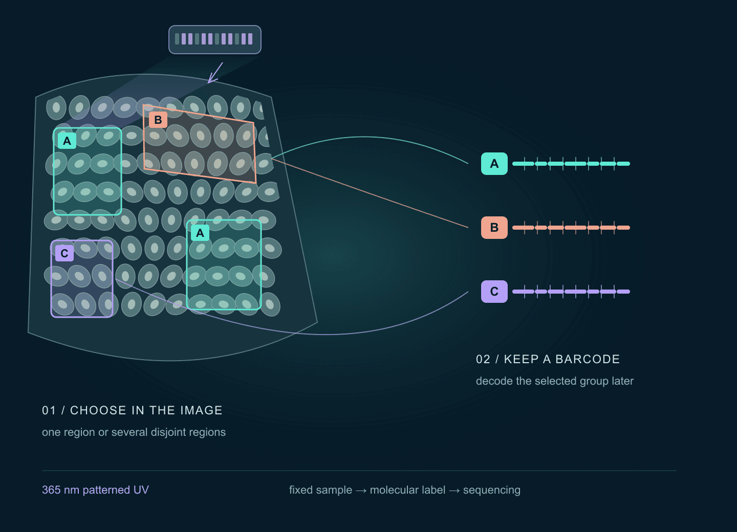
Connect regions selected in a tissue image to molecular barcodes and sequencing. Explore the published Light-Seq application, a barcode-group lab, registration geometry and the Polygon optical setup.
Open guide Optogenetics
Plan targeted illumination in neuronal cultures or tissue slices: compare Polygon inputs, register camera ROIs, verify delivered light, and synchronize electrophysiology or compatible imaging. Includes an interactive pattern illustration.
Open guide Nonlinear microscopy
Signal scales as P²/(τ·f), so the pulse your objective stretches from 100 fs to 300 fs costs two thirds of your fluorescence at identical average power. The beam path, part by part, and an interactive excitation budget.
Open guide