01 · Start with the measurement
Focusing is not scanning. Decide which one the image needs before deciding what moves.
A Z-stack and a lateral scan ask for different things. Moving the objective axially changes which plane of a stationary specimen is in focus; it cannot move the field sideways, tile a larger area, or raster a beam across a sample. Lateral scanning needs the sample or the objective to translate in X and Y, with the axis of motion parallel to the image plane and repeatable to a fraction of a pixel. Systems that need both have to provide both, and the question is then which assembly carries each.
The central decision is not which stage is best but which moving assembly best preserves the experiment while meeting travel, stability and timing. Moving the sample keeps the optical train fixed and aligned but moves everything attached to the sample. Moving the objective keeps the specimen, its medium, its tubing and its probes untouched but puts a few hundred grams of glass and brass on a piezo and moves it through the immersion film. A combination puts coarse travel under fine travel and asks two controllers to agree on timing.
Z-stacks
A series of planes through the specimen. Needs axial travel of the stack depth with a repeatable step, and settling fast enough that the stack finishes before the specimen changes. Either the objective or the sample can provide it.
Autofocus and focus hold
Small, frequent axial corrections driven by a focus sensor. Needs bandwidth and resolution more than travel, and a controller that accepts an analog or software setpoint quickly.
Lateral raster scanning
Moving the field over the specimen in X and Y at nanometre steps: stage-scanning confocal, AFM-style correlative work, super-resolution tiling. Only a lateral sample or objective stage provides this; an axial focuser cannot.
Drift correction
Slow XYZ corrections from fiducial tracking over minutes to hours. Needs closed-loop sub-10 nm repeatability in three axes and low self-heating, not speed.
Multi-position imaging
Visiting many fields millimetres apart. Needs coarse travel with good return accuracy, then fine focus at each site. A piezo scanner alone cannot reach the positions; a motor stage alone cannot focus finely.
Combinations
Most real systems combine two of the above. The choice of what moves is then a choice of which requirement gets the stiffest, lightest path.
For the mechanisms behind the stages named in this guide — flexure scanners against stick-slip motors, and open loop against closed loop — see our guides on piezo drive architectures, open-loop versus closed-loop piezo control and choosing a precision positioning stage. This article stays with the microscope.
02 · Sample scanning versus objective focusing
Four arrangements, no universal winner.
The same nanometre-class motion can be put under the sample, under the objective, or split between a millimetre stage and a micrometre scanner. Each arrangement moves a different mass, disturbs a different part of the experiment and settles at a different rate.
| XY / XYZ sample positioning | Z-only sample positioning | Piezo objective focusing | Coarse + fine combination | |
|---|---|---|---|---|
| Motion axes and usable travel | X, Y and Z; 100–300 µm per axis in the clear-aperture scanners, up to 500 µm in single-axis modules | Z only; 100–200 µm on clear-aperture stages, 100–300 µm on compact modules | Z only; 100, 200 or 400 µm at the objective | Millimetres in XY from a piezo-motor stage, plus 100–400 µm of fine motion from a scanner or objective focuser |
| Moving mass and mechanical load | Sample, holder, insert, any medium; resonance falls with every gram (Carrier.S200.XYZ: 155/155/320 Hz unloaded, 120/120/200 Hz at 350 g) | Same load, one axis; stiffer and faster for the same mass | Objective only, typically 150–400 g; resonance quoted at 150 g (250 Hz for OB100, 560 Hz for OBHL100) | Coarse stage carries scanner plus sample; fine stage carries only sample |
| Sample access and mounting | Clear aperture 66 × 66 or 77 × 65 mm for transmitted light; insert must be rigid and light | Aperture 80 × 80 mm on Carrier.S Z stages; simple to add under an existing insert | Sample untouched: dishes, chambers, tubing and probes stay where they are | Aperture set by the coarse stage (20 × 20 to 120 × 120 mm depending on model) |
| Objective compatibility | Any objective; nothing changes at the nosepiece | Any objective | M25 × 0.75 thread on the scanner; RMS, M27 and others through an adapter that adds height and mass | As for the fine element chosen |
| Immersion conditions | Objective fixed; oil or water film is sheared by lateral motion, which can drag a loose coverslip | Sample lifts toward a fixed objective; the film thickness changes with Z | Objective moves through the film; viscous coupling adds damping and can disturb a floating dish or open bath | Combination of the above |
| Settling and acquisition timing | Slowest axis sets the plane rate; XY settling limits tile rates | One axis, faster settling than a stacked XYZ of equal load | Fastest axial option for a light objective; response time 5–24 ms per the datasheets | Coarse moves take hundreds of milliseconds to seconds; fine motion as above |
| Integration complexity | Stage plate adapter, insert, three cables, three controller channels | One channel; usually fits under an existing insert | Thread adapter, turret clearance, parfocal shift, one channel | Two controller families, two SDKs, two trigger paths |
| Typical applications | Stage-scanning confocal and super-resolution, correlative AFM/optical, small rigid samples | Z-stacks on inverted systems with sealed chambers; focus hold | Z-stacks and autofocus where the specimen must not move: live cells, patch clamp, microfluidics | High-content and multi-position imaging, slide scanning with fine focus |
| Limitations | Heavy or liquid samples slow it down; tubing and probes move with the sample | No lateral scanning; heavy loads | No lateral scanning; objective mass and immersion drag; focus shift across index mismatch applies to any axial focuser | Return accuracy of the coarse stage sets tile registration; more to synchronise |
Figures are from the manufacturer’s 2025 ambient catalogue for the models named in section 07; loaded resonances are quoted at the load the datasheet used.
03 · When moving the sample makes sense
Move the sample when the optics are the expensive, aligned part.
Lateral scanning. Stage-scanning confocal, correlative AFM and optical work, structured-illumination and localisation tiling all move the field over the specimen with the beam path fixed. With the sample on the scanner, the illumination and detection optics never see a changing pupil, the point-spread function is the same at every position, and the scan is limited only by the stage. Light-sheet microscopy has worked this way since the first SPIM instruments translated the specimen through a stationary sheet.
Small rigid specimens. A coverslip, a chip, a fibre or a cantilever weighs tens of grams with its holder and can ride on a compact serial scanner or a parallel-kinematic module at its unloaded resonance. This is where 700 Hz axes and sub-nanometre resolution actually apply.
Fixed optical assemblies. Custom-built systems, two-objective geometries, or objectives fitted with correction collars and piezo-driven elements of their own are better left alone; put the motion under the sample.
XYZ sample control. When the experiment needs a defined position in three axes with a clear optical path for transmitted light, the clear-aperture Carrier.S XYZ stages carry an insert over a 66 × 66 mm aperture with 100–300 µm of travel per axis and 5 kg of static payload.
What moving the sample drags along
- Heavy chambers and incubators: every gram lowers the loaded resonance and lengthens settling. The Carrier.S200.XYZ.C falls from 155/155/320 Hz unloaded to 120/120/200 Hz with 350 g; a 2 kg chamber is off the published curve.
- Liquid samples: an open dish sloshes; a sealed chamber shifts its centre of mass. Lateral moves excite surface waves that take longer to die than the stage does.
- Tubing, perfusion lines, heater and electrode cables: each one is a spring attached to the moving platform and a source of hysteresis the sensor cannot see.
- Electrical probes and patch pipettes: they are referenced to the fixed frame, so moving the sample moves the specimen relative to the probe. This is the classic reason to focus the objective instead.
- Delicate specimens: acceleration at the start and end of each step is a mechanical stimulus; embryos, hydrogels and suspended cells notice it.
Sample-stage families
- Carrier.S100.XYZ.C, Carrier.S200.XYZ.C, Carrier.S300.XYZ.C — clear-aperture XYZ, 66 × 66 mm aperture, 150 × 150 × 30 mm, 5 kg (3 kg for S300).
- Carrier.SL200.XY.C, Carrier.SL200.XYZ.C — 19.5 mm-high XY or XYZ with a 77 × 65 mm aperture, made to sit on a Carrier.L piezo-motor stage.
- Carrier.S100.Z.C, Carrier.S200.Z.C — Z only, 80 × 80 mm aperture, 5 kg.
- S100.XYZ.C, S200.XYZ.C, S100.XYZ.C.P — 55 × 55 mm serial or 40 × 40 × 40 mm parallel modules for small, rigid samples without a through-aperture.
- SH30.XYZ.C — 30 × 30 × 15 µm with 10 kg payload for heavy fixtures, 500 Hz unloaded.
All pair with the MC-Archimedes.N scanner controller, one .C channel per axis. Browse the full ambient piezo catalogue.
04 · When moving the objective makes sense
Move the objective when the specimen must not know it is being imaged.
Z-stacks and autofocus. A piezo objective scanner threads between the nosepiece and the objective and moves the objective by 100, 200 or 400 µm with a capacitive sensor closing the loop. Nothing on the stage moves: perfusion, heating, patch electrodes, microfluidic connections and the dish itself stay where they were set. Response times of 5–24 ms on the objective scanners here make it the fastest axial option for a light objective, and the same device serves a focus-hold loop driven from a focus sensor through the controller's analog input.
Mass and resonance. The objective is the payload. A high-NA immersion objective is typically 150–400 g, and the datasheet resonance is quoted at 150 g: 250 Hz for the OB100, 165 Hz for the OB400, 560 Hz for the high-load OBHL100. Heavier objectives push the resonance down the curve in section 05, and the settle time up.
Thread, adapters and clearance. The scanners carry an M25 × 0.75 mount, which fits Nikon CFI and Leica HC objectives directly; RMS (0.8″-36) and M27 × 0.75 (Olympus, Zeiss) objectives need an adapter that adds height and a few grams. Any objective scanner adds height between turret and objective, which shifts the parfocal position, may collide with neighbouring objectives when the turret rotates, and has to fit under the stage on an inverted frame. Check the turret clearance with the scanner's drawing before ordering, and plan for the coarse focus to absorb the added height.
Orientation and cabling. On an inverted microscope the scanner works against gravity plus the objective; on an upright it works with it. The cable leaves the scanner body sideways and must clear the turret through its full rotation; route it with a loop so it neither pulls on the scanner nor rubs on the frame.
Immersion and the specimen. Moving an oil or water objective moves it through its immersion film. Viscous coupling adds damping the datasheet did not include and can tug a floating coverslip or an open bath. Across a refractive-index mismatch the focal plane inside the specimen moves by roughly nsample/nimmersion times the mechanical step for any axial focuser, sample or objective; the stack spacing you set is not the spacing you get in a watery sample under oil.
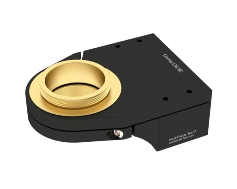
Objective-scanner family
- Carrier.OB100.C — 100 µm, 1 nm, 15 ms response, 600 / 250 Hz (unloaded / 150 g), 0.5 N/µm.
- Carrier.OB200.C — 200 µm, 3 nm, 19 ms, 480 / 220 Hz, 0.35 N/µm.
- Carrier.OB400.C — 400 µm, 5 nm, 24 ms, 380 / 165 Hz, 0.25 N/µm, 350 g.
- Carrier.OBHL100.C — 100 µm, 1 nm, 3 nm repeatability, 5 ms, 1 kHz / 560 Hz, 3 N/µm, 500 g.
- Carrier.OB200.XY.C — lateral objective scanning, 200 × 200 µm, 20 mm clear aperture, 500 g payload.
All specify the MC-Archimedes.N controller with .C capacitive channels and offer .NM, .HV and .UHV variants. Thread adapters and autofocus integration are configured with us rather than listed as catalogue parts; treat them as items to confirm.
05 · Translate imaging requirements into stage specifications
The datasheet describes an unloaded stage on a bench. Your microscope is neither.
| Specification | What it means for the image | What to watch |
|---|---|---|
| Field of view and scan depth | Lateral travel must cover the field or tile you want to build with margin; axial travel must cover the thickest specimen plus focus drift and the difference in parfocal position between objectives. | Closed-loop travel is smaller than open-loop travel on the same stage (S100 series: 100 µm closed, 120 µm open). Order against the closed-loop figure. |
| Usable closed-loop travel | The range over which the sensor is linear and the controller can hold position. The datasheet linearity (0.03 % of travel on the scanners here) is the residual after the controller’s linearisation, over the full closed-loop range. | Travel at the ends of range costs the most force and settles slowest; leave 5–10 % unused. |
| Resolution, repeatability, accuracy, stability | Resolution is the smallest commanded step the system responds to (0.2–1 nm open loop, 1–5 nm closed loop on these scanners). Repeatability is how close it returns to a position (10 nm on most Carrier and S scanners, 3 nm on OBHL100). Accuracy is closeness to the true position and depends on calibration, mounting and temperature. Stability is drift over the measurement time and is mostly thermal. | A 1 nm commanded step is not a 1 nm accurate move. The image, not the controller readback, is the reference. |
| Payload and loaded resonance | Adding mass lowers the first resonance roughly as f = f₀·√(m_eff/(m_eff + m)). The datasheets give two points (unloaded and at 150 g or 350 g); anything heavier is an extrapolation. | Payload rating is a static limit. A stage at its rated payload may resonate below 100 Hz and settle in tens of milliseconds. |
| Settling time and closed-loop bandwidth | Usable closed-loop bandwidth is a fraction of the loaded resonance, commonly a third to a tenth depending on damping and tuning; settling to within tolerance takes several periods of that bandwidth. | Resonance frequency is not imaging speed. A 250 Hz loaded objective scanner does not take 250 planes per second; the datasheet response time (15 ms for OB100) is a better first estimate, and the measured settle on your system is the real one. |
| Cross-axis motion, tilt and sensor placement | Every axis moves a little in the others: pitch/yaw of ±10–30 µrad on the objective scanners, Z–XY crosstalk of ±30–50 nm on the Carrier.S XYZ stages. Capacitive sensors on these scanners measure the moving platform directly (“direct metrology”), so what is controlled is the platform, not the actuator. | The sample sits above the sensor plane. Tilt times the distance to the focal plane is a lateral error the loop cannot see (the Abbe offset); keep the sample low. |
| Controller compatibility and drive current | Scanners with capacitive sensors pair with MC-Archimedes.N .C channels (−20…150 V, 24 W per channel, 20/50 kHz sensor sampling). Piezo-motor stages pair with MC-Newton.S or MC-Newton.MSx (0–75 V, optical encoder). Drive current sets how fast a given capacitance can be slewed, which is where scan speed is actually limited for large stages. | One channel per axis; a three-axis scanner needs a three-channel controller. Do not pair a scanner with a motor controller or the reverse. |
Resonance is not imaging speed
A 250 Hz loaded scanner has a closed-loop bandwidth well below 250 Hz and settles in several periods of that. Planes per second come from settle plus exposure plus readout, not from the resonance line.
A commanded step is not an accurate move
The controller will report the step it commanded; the sensor will report the platform; the image reports the specimen. Only the last one includes tilt, thermal drift and the holder’s compliance.
Unloaded specifications describe a bench
Add the insert, the dish, the medium and the cables, then re-derive resonance, settle time and the force needed for the step. Ask us for the loaded figures when the datasheet does not give them.
06 · Synchronise motion and image acquisition
A stack is a schedule. Write it down before you buy the stage.
Step-and-settle moves the stage, waits until it is within tolerance, exposes, reads out, and repeats. It is simple, and the image is taken with the stage stationary. Continuous scanning drives the stage with a ramp and exposes while it moves; it is faster and avoids the settle, but the motion during exposure has to be small against the axial resolution, and the position must be recorded — from the sensor, through the controller's trigger output or its readback — to know where each frame was taken. Piezo-motor stages step; flexure scanners with an analog input can do either.
Triggering. Either the controller fires the camera when the stage has settled (position-triggered), or the camera's exposure-end fires the next move (camera-master). The MC-Archimedes.N and MC-Newton controllers expose SMA TTL trigger lines and a 0–10 V analog input for exactly this. Camera-master is the easier one to get right, because readout can then overlap the next move.
Position feedback from the capacitive sensor tells you where the platform was; it does not tell you where the specimen was if the holder flexed, and it does not know about immersion drag. Use it to verify the schedule, and use the image — a bead, a fiducial, a sharp edge — to verify the position.
Worked example: a 50-plane stack with an objective scanner
- Assumptions. 50 planes at 0.3 µm (15 µm stack, within the 100 µm of an OB100); one channel; move-and-settle of 20 ms per step with the objective fitted (the datasheet response time is 15 ms; 20 ms is an assumed measured value, not a specification); 30 ms exposure; 10 ms full-frame readout on a triggered sCMOS.
- Sequential. Each plane pays 20 + 30 + 10 = 60 ms; the stack takes 50 × 60 ms = 3.0 s.
- Overlapped. Readout runs during the next move, so each plane pays 30 + max(20, 10) = 50 ms; the stack takes 50 × 50 + 10 = 2.51 s. Exposure is 60 % of the time; the stage is the next thing to speed up, not the camera.
- Two channels sequentially per plane. Overlapped: 2 × 30 + 10 + 20 = 90 ms per plane, 4.51 s per stack — the second readout cannot hide behind a move that has not started.
- What is not in the number. Software latency between frames, trigger jitter, illumination switching and any autofocus step. Measure a real stack and compare before you promise a frame rate.
Acquisition-time estimator
Z-stack and multi-position timing
Move-and-settle, exposure and readout per plane, with or without readout overlapping the next move. Enter the settle time you measured on the installed stage, not a datasheet resonance.
Stack depth ÷ step size. The step size itself does not enter the time.
Time to arrive within your tolerance, measured with the real objective or sample on the stage.
Full-frame readout time from the camera datasheet, or the interval a detector needs before the next trigger.
Sequential channels before the stage moves on.
Estimate
2.51 s
one 50-plane stack
- Sequential stack
- 3.00 s
- Overlapped stack
- 2.51 s
- Planes per second
- 19.9
- Time spent exposing
- 60 %
An estimate of the acquisition schedule, not a guaranteed product performance.
- Assumes a constant settle time per plane; large steps, direction reversals and a heavier load all lengthen it.
- Ignores software latency, trigger jitter, autofocus loops, filter changes and illumination switching.
- Overlap requires a camera that reads out while armed for the next trigger and a controller that starts the move on the exposure-end signal.
- Settle time must be measured on your installed system against your image-quality tolerance.
07 · Three practical configurations
The decision, three times, with part numbers.
Each configuration is drawn from listed models and their published figures. The diagrams are conceptual; the third follows a combination the manufacturer publishes, the first two are illustrative arrangements. The last block of each is what has to be confirmed before it becomes an order.
Z-stack imaging of live cells on an inverted microscope
Requirement. 20–40 µm stacks through cells in a perfused, heated dish with a patch pipette in place; 0.3 µm steps; two channels; the dish and the pipette must not move.
Why the objective. Everything attached to the sample is a reason not to move it. A 100 or 200 µm objective scanner covers the stack with margin and leaves the microscope's own XY stage for coarse positioning.
Products. Carrier.OB100.C (100 µm, 1 nm, 15 ms) or Carrier.OB200.C (200 µm, 3 nm, 19 ms); Carrier.OBHL100.C if the objective is heavy or the stack rate is the priority. Controller: MC-Archimedes.N with one .C channel, TTL trigger to and from the camera, USB or Ethernet to the acquisition PC.
Mounting. M25 × 0.75 direct for Nikon and Leica; adapter for Olympus, Zeiss or RMS. On an inverted frame the scanner sits under the stage and the objective points up through it; the scanner body (see its drawing) plus any adapter must clear the stage underside and the turret.
Tradeoffs. Oil or water coupling damps the scanner and can tug the dish; the focal step inside an aqueous sample under oil is, paraxially, about 0.88× the mechanical step; the objective's mass sets the loaded resonance and the settle time, which must be measured with that objective.
Confirm. Objective thread, mass and parfocal length; turret clearance with the scanner fitted; whether the other objectives remain usable; camera trigger polarity; measured settle at your step size.
Stage-scanning and localisation microscopy beneath a fixed objective
Requirement. Raster a 100 × 100 µm field with nanometre steps under a fixed high-NA objective, hold a fiducial to within 10 nm in XYZ over an hour, and keep transmitted-light illumination through the sample.
Why the sample. Lateral scanning is the requirement, so an axial focuser cannot do it. A fixed objective keeps the point-spread function constant across the scan; the clear aperture keeps the condenser in play.
Products. Carrier.S100.XYZ.C (100 µm per axis, 1 nm, 10 nm repeatability, 66 × 66 mm aperture, 5 kg static) or Carrier.S200.XYZ.C for 200 µm; for a slide on a light insert the 19.5 mm-high Carrier.SL200.XYZ.C; for a coverslip-sized rigid sample without transmitted light, S100.XYZ.C.P (40 mm cube, 700 Hz, 200 g). Controller: MC-Archimedes.N with three .C channels; analog input for scan waveforms; TTL to the detector.
Mounting. Bolt the stage to the microscope stage plate through an adapter plate matched to your frame, keep the insert as light and stiff as possible, and route the three cables in a loop that does not touch the frame. The 30 mm height of the Carrier.S stages must fit under the objective at focus with the coarse stage in range.
Tradeoffs. Loaded resonance and settle depend on the insert (155/155/320 Hz unloaded to 120/120/200 Hz at 350 g for the S200); Z–XY crosstalk of ±30 nm at full travel; the holder's thermal drift adds to the stage's; probes referenced to the frame move relative to the specimen.
Confirm. Stage-plate pattern and available height; insert mass with medium; aperture against the condenser and its working distance; cable exits; whether closed-loop travel (100 µm) or open-loop travel (120 µm) is the number you designed to.
Multi-position imaging with fine focus at every site
Requirement. Visit 40 positions across a 100 × 100 mm area every ten minutes, take a short stack at each, and register the tiles to a few hundred nanometres.
Why the combination. No piezo scanner reaches 100 mm and no piezo-motor stage focuses at nanometre repeatability. The manufacturer publishes this exact pairing for microscopy: a Carrier.L1010s.XY for coarse travel, a Carrier.SL200.XYZ.C for fine scanning, and a Carrier.OB400.C for objective focusing.
Products. Carrier.L1010s.XY (100 × 100 mm, 10 nm minimum incremental motion, 4 kg, 20 × 20 mm full-travel aperture) or Carrier.L1010.XY (120 × 120 mm aperture) where transmitted light matters; Carrier.SL200.XYZ.C for fine XYZ; Carrier.OB400.C for 400 µm of objective focus. Controllers: MC-Newton.MSx with two channels for XY and MC-Archimedes.N with four .C channels for the piezo axes, both on the PC with TTL to the camera.
Mounting. The SL200 is documented as compatible with the Carrier.L7550.XY; the L1010s combination is shown in the catalogue's microscopy example. The stack is 28 mm (L1010s) plus 19.5 mm (SL200) plus the insert above the stage plate.
Tradeoffs. Coarse moves at up to 10 mm/s take seconds across the plate; tile registration depends on the coarse stage's bidirectional repeatability, which is not published — plan a visit order that approaches each site from the same direction, or register on image features. Two controller families mean two SDKs and two trigger paths.
Confirm. Mounting space (285 × 285 mm for the L1010s); aperture against your illumination; total height under the objective; repeatability at your visit pattern; whether one shared scan-controller setting suits all sites.
Product selection table
From requirement to model number, with the conditions attached.
Every figure is from the manufacturer's 2025 ambient catalogue; loaded resonances name the load they were measured at. Stage–controller pairings are the ones the datasheets specify. The system builder walks the same choices and adds them to an enquiry.
| Requirement | Product | Documented specification | Documented controller | Confirm before ordering |
|---|---|---|---|---|
| Z-stacks and autofocus by moving the objective | Carrier.OB100.C / Carrier.OB200.C / Carrier.OB400.C | 100 / 200 / 400 µm closed-loop; 1 / 3 / 5 nm closed-loop resolution; 10 nm repeatability; 0.03 % linearity; ±10/20/30 µrad pitch-yaw; 15 / 19 / 24 ms response; 600/480/380 Hz unloaded, 250/220/165 Hz at 150 g; 270–350 g; M25 × 0.75; capacitive sensor | MC-Archimedes.N with one .C channel | Objective thread and mass; turret clearance and added height; parfocal shift; immersion coupling to the sample. |
| Faster or heavier objective focusing | Carrier.OBHL100.C | 100 µm; 1 nm closed-loop; 3 nm repeatability; 5 ms response; 3 N/µm stiffness; 1 kHz unloaded, 560 Hz at 150 g; 500 g; M25 × 0.75 | MC-Archimedes.N .C | Its own 500 g mass on the nosepiece; whether the turret can carry it; clearance to neighbouring objectives. |
| Lateral objective scanning with the sample fixed | Carrier.OB200.XY.C | 200 × 200 µm; 2 nm closed-loop; 10 nm repeatability; 20 mm clear aperture; 70 × 70 × 25 mm; 350 Hz unloaded; 500 g payload; 280 g | MC-Archimedes.N with two .C channels | Optical path through the 20 mm aperture; mounting between turret and objective; pupil shift from lateral objective motion. |
| XYZ sample scanning with transmitted-light access | Carrier.S100.XYZ.C / Carrier.S200.XYZ.C / Carrier.S300.XYZ.C | 100 / 200 / 300 µm per axis; 1 / 1.5 / 2 nm closed-loop; 10 nm repeatability; 66 × 66 mm aperture; 150 × 150 × 30 mm; resonance 180/180/390, 155/155/320, 135/135/250 Hz unloaded and 150/150/250, 120/120/200, 90/90/140 Hz at 350 g; payload 5 / 5 / 3 kg; Z–XY crosstalk ±30–50 nm | MC-Archimedes.N with three .C channels | Stage-plate mounting pattern; insert mass; 30 mm added height under the objective; cable exit. |
| Low-profile XY or XYZ sample scanning on a motorised stage | Carrier.SL200.XY.C / Carrier.SL200.XYZ.C | 200 µm per axis; 2 nm closed-loop; 10 nm repeatability; 77 × 65 mm aperture; 182 or 190 × 150 × 19.5 mm; 500 g payload; documented as compatible with Carrier.L7550.XY | MC-Archimedes.N with two or three .C channels | Insert and sample under 500 g; loaded resonance (not published — measure); combination bracket to the coarse stage. |
| Compact XYZ scanning of a small rigid sample | S100.XYZ.C / S200.XYZ.C / S100.XYZ.C.P | 100 or 200 µm per axis; 1 / 1.5 nm closed-loop; 55 × 55 × 40–45 mm serial stack (400/350/300 or 300/250/200 Hz), or 40 × 40 × 40 mm parallel-kinematic .P with 700 Hz all axes, 10 nm repeatability and 200 g payload | MC-Archimedes.N with three .C channels | No clear aperture on the serial modules; sample must be mounted on top; payload of the .P version is 200 g. |
| Z-only sample focusing under an existing insert | Carrier.S100.Z.C / Carrier.S200.Z.C or S100.Z.C / S300.Z.C | Carrier.S Z: 100 / 200 µm; 1 nm; 10 nm repeatability; 80 × 80 mm aperture; 500/200 or 350/120 Hz (unloaded / 2.5 kg); 5 kg. S Z modules: 100 / 300 µm; 0.5 / 1 nm; 55 × 55 × 18 mm; 700 / 320 Hz; 500 g | MC-Archimedes.N with one .C channel | Pitch/yaw of the Z modules (±100–200 µrad) against your field; aperture against the condenser. |
| Coarse XY travel for multi-position imaging | Carrier.L7550.XY / Carrier.L1010.XY / Carrier.L1010s.XY | 75 × 50 / 100 × 100 / 100 × 100 mm travel; 10 nm minimum incremental motion; 2 nm optical encoder; apertures 85 × 65 / 120 × 120 / 20 × 20 (50 × 50 over 70 × 70 mm) mm; ~15 / 10 / 10 mm/s; payload 2 / 4 / 4 kg; 0.3 mrad pitch-yaw; self-locking | MC-Newton.MSx (2 channels) or two MC-Newton.S | Bidirectional repeatability at your visit pattern (only minimum incremental motion is published); mounting space (up to 350 × 350 mm); aperture versus your illumination. |
| Coarse Z under a piezo stage or for parfocal changes | LS35z.Lab / LS65z.Lab / LS80z.Lab | 10 mm travel; 10 nm minimum incremental motion; ±150 nm unidirectional repeatability; 500 g / 500 g / 1 kg payload; 35 × 35 × 41, 65 × 65 × 44, 80 × 80 × 40 mm | MC-Newton.S | Payload includes everything above the stage; self-locking hold with power off is a feature, but confirm creep over your imaging time. |
| Controllers | MC-Archimedes.N · MC-Newton.S · MC-Newton.MSx | Archimedes.N: ≤ 8 channels, FPGA, .C capacitive or .S strain-gauge, 20/50 kHz sensor sampling, −20…150 V, 24 W per channel, 0–10 V analog in, SMA TTL trigger, USB/Ethernet, GUI + SDK. Newton.S: 1 channel, 0–75 V, 30 W, optical encoder, USB/Ethernet/RS485, TTL trigger. Newton.MSx: up to 10 channels, 100 W total, EtherCAT on request | — | Channel count equals axes; sensor suffix matches the stage; trigger polarity and SDK against your acquisition software. |
08 · Purchasing checklist
Nine things we need before we can name a configuration.
01
Sample dimensions and mass
Including holder, dish, medium, lid, tubing and probes; note whether it is liquid-filled or delicate.
02
Objective model and mass
Thread (RMS, M25 × 0.75, M27 × 0.75), parfocal length, immersion type, and whether other objectives on the turret must stay usable.
03
Required axes and what moves
X, Y, Z or a subset; sample, objective or both; whether lateral scanning is needed at all.
04
Travel per axis
Fine (µm) with margin; coarse (mm) for multi-position; stack depth including drift and parfocal differences.
05
Imaging mode
Z-stack, autofocus, raster scan, drift correction, multi-position, time-lapse; camera or point detector; exposure and readout times.
06
Target acquisition time
Planes per stack, stacks per minute, positions per run; which operations may overlap.
07
Feedback requirements
Closed loop and sensor type; repeatability and stability over the run; whether the image will be the reference.
08
Available space
Stage-plate aperture and pattern, height under the objective, turret clearance, cable exits.
09
Synchronisation interface
TTL trigger direction, analog scan input, SDK language, EtherCAT or Ethernet, software you already use.
The contact form opens pre-filled with these nine lines; answer what you can and we will ask for the rest.
Send the checklistSources and references
- Zolix / MultiFields, Piezo Stages — Ambient Environment, 2025 catalogue — specifications of the Carrier.OB, Carrier.S, Carrier.SL, S, SH, Carrier.L and Lab series, the MC-Archimedes.N and MC-Newton controllers, and the published microscopy combination (Carrier.L1010s.XY + Carrier.SL200.XYZ.C + Carrier.OB400.C).
- Pawley (ed.), Handbook of Biological Confocal Microscopy, 3rd ed., Springer (2006) — stage scanning versus beam scanning, axial sampling and focus drift in practice.
- Hell, Reiner, Cremer & Stelzer, Aberrations in confocal fluorescence microscopy induced by mismatches in refractive index, Journal of Microscopy 169, 391–405 (1993) — focal shift and aberration when focusing across an index mismatch.
- Huisken, Swoger, Del Bene, Wittbrodt & Stelzer, Optical sectioning deep inside live embryos by selective plane illumination microscopy, Science 305, 1007–1009 (2004) — sample translation through a stationary light sheet.
- McGorty, Kamiyama & Huang, Active microscope stabilization in three dimensions using image correlation, Optical Nanoscopy 2, 3 (2013) — fiducial-based XYZ drift correction with a piezo stage.
- Fleming & Leang, Design, Modeling and Control of Nanopositioning Systems, Springer (2014) — loaded resonance, closed-loop bandwidth, settling and sensor placement in flexure nanopositioners.
- Slocum, Precision Machine Design, Prentice Hall (1992) — Abbe offset: tilt at the stage becomes lateral error at the sample.