Back to Home
← All guides

Integrated photonics · 28 min

Fibre-to-chip alignment: choosing stages, feedback, and fixation

From coupling geometry and mode-field tolerance to the positioning architecture, feedback loop, search workflow, and adhesive cure that turns a laboratory measurement into a permanent package.

Edge vs gratingTolerance → motionStage selectionOptical feedbackFirst lightUV fixation3 configurations
Six-axis fibre alignment stage with crossed-roller guides for photonic chip coupling
fibre → PIC → detector → controller → stage

1 · Define the coupling interface

The coupling scheme decides the alignment geometry.

Edge coupling brings the fibre to the chip facet, coaxial with the waveguide. The hard alignment axis is lateral XYZ: small, well-matched modes make the transverse peak narrow and the longitudinal gap matters as the beam diffracts.

Grating coupling brings the fibre from above at the design angle. Lateral capture is comparatively generous because the grating is designed to match the fibre mode size, but the phase-matching condition punishes angular error — the angle, not the position, is the critical axis.

Single fibres, lensed fibres, and fibre arrays each change the problem again. A lensed fibre shrinks the mode and tightens lateral tolerance. A fibre array adds the constraint that angular errors misalign outer channels even when the centre is coupled. Identify the coupling scheme, fibre type, port count, and whether attachment is temporary or permanent before selecting equipment.

ConsiderationEdge couplerGrating coupler
Approach geometryFibre approaches the chip facet horizontally, aligned coaxially with the waveguide.Fibre approaches from above at the grating design angle, typically 8–15° from vertical.
Hard alignment axisLateral (X/Y). Small matched modes make the transverse peak narrow; Z gap adds diffraction loss.Angle (θ). Phase matching punishes angular error; lateral capture is comparatively generous.
Fibre type influenceLensed or UHNA fibre reduces mode mismatch and tightens lateral tolerance further.Standard cleaved SMF is typical; the grating is designed to match its mode size.
Fibre arraysV-groove array butt-coupled to an edge-port array. Pitch accuracy and angular alignment affect all channels simultaneously.Fibre array pressed above grating array at uniform angle. Pitch and planarity control coupling across channels.
Working distanceNear-zero. The fibre or lens tip is within a few micrometres of the facet.Larger. Typically tens of micrometres above the chip surface, easing clearance.
Permanent attachmentAdhesive applied at the chip edge; access for UV cure may be restricted by the fibre approach.Adhesive applied from the side or above; vertical fibre gives better curing access.

Temporary vs. permanent. A laboratory measurement needs repeatable alignment and may tolerate a few minutes of setup per device. Permanent packaging additionally requires adhesive placement, UV cure access, shrinkage compensation, fixture release, and post-cure verification — all of which impose additional mechanical and optical constraints on the station.

2 · Translate tolerance into motion

Optical mode size sets the positioning budget.

The coupling between two optical modes depends on their spatial overlap. Four displacement terms degrade it independently:

Lateral offset (d):
Transverse misalignment perpendicular to the optical axis. This is usually the tightest tolerance for a well-matched edge coupler.
Axial separation (z):
Longitudinal gap between fibre and chip. The beam diffracts across the gap, so coupling drops with increasing distance.
Angular tilt (θ):
Pointing error of the fibre axis relative to the waveguide. For grating couplers, the phase-matching condition makes this the dominant loss term.
Mode mismatch:
Unequal mode-field diameters. This baseline loss cannot be removed by alignment — only by changing the fibre or adding a spot-size converter.

When modes are well matched and small (1–3 µm MFD), the lateral 1 dB tolerance can be a fraction of a micrometre. A useful search step is about one tenth of that tolerance, so the controller samples the peak instead of jumping across it.

Five positioning specifications

Capture range
Total travel available for initial approach and search — typically millimetres.
Resolution
Smallest controllable position increment — nanometres for a piezo, micrometres for a micrometer.
Repeatability
Variation when returning to the same commanded position. Determines whether a peak can be re-found reliably.
Accuracy
Error between commanded and true position. Less critical for peak search (which uses optical feedback) than for fixture-based assembly.
Long-term stability / drift
Position change over time from thermal expansion, creep, or relaxation — critical during cure and extended sweeps.

Interactive

See how mode size and offset shape the coupling peak.

Adjust the fibre and chip mode-field diameters to see how lateral misalignment degrades coupling efficiency. The 1 dB tolerance and suggested search step update in real time.

Coupling tolerance vs. lateral offset

Adjust the mode-field diameters to see how lateral misalignment degrades coupling. The plot shows additional loss beyond the mode-mismatch baseline.

Mode-mismatch loss

0.02 dB

1 dB tolerance

±0.74 µm

3 dB tolerance

±1.29 µm

Search step (≈1/10)

74 nm

051015202530012345Lateral offset (µm)Total loss (dB)1 dB3 dBbaseline 0.0 dB
Educational model only. This visualisation assumes two co-axial, circularly symmetric Gaussian modes and plots only the lateral-offset term. It does not apply to grating couplers (where angular phase matching dominates), lensed fibres with aberration, fibre arrays, or any specific PIC fabrication process. Use it to build intuition about mode-size tolerance, not to predict coupling for a real device.

3 · Choose axes and stage architecture

Match the motion architecture to the coupling problem.

Four approaches, from simplest to most capable. Most practical stations combine a coarse stage for capture with a fine stage for the peak.

Manual fibre-alignment stages

Micrometer-driven XYZ (and optional angle) with sub-micrometre sensitivity. Fast to set up, simple, no electronics. The operator is the feedback loop. Limited by hand sensitivity — typically 0.5–2 µm — and cannot hold a peak during a long sweep.

Motorized positioning

Stepper-motor drives (DNXP-A for NXP platforms, or Lab/Indus piezo motors) enable remote coarse approach and automated search sequences. Step resolution is 0.625–1.25 µm for stepper drives; 10 nm for piezo motor stages. Add a fine piezo scanner for the final peak.

Coarse + fine piezo

Combine a manual or motorized coarse stage with a closed-loop piezo scanner (S100.XYZ.C, NXP-NP). The coarse stage provides millimetres of capture; the piezo provides nanometre peak search and hold. This is the standard topology for active-alignment stations.

Multi-axis flexure / parallel platforms

Six-degree-of-freedom parallel-kinematic platforms (NXP-6NP, Free6D) control translation and rotation from a common centre. Essential for fibre arrays and multi-port devices where angular errors propagate across channels.

When angular axes become necessary. XYZ is sufficient when the fibre approach is mechanically fixed and the coupling scheme is tolerant of small angular errors. Add pitch, yaw, or roll when the coupler design demands a specific incidence angle (grating), when the chip facet is not perpendicular, or when aligning a fibre array — where 0.1° of tilt at the centre can misalign an outer channel by several micrometres over a 250 µm pitch.

Stage family decision table

Map your alignment requirements to the Precisometer stage families. Each column shows capability; the note column explains the engineering reason.

RequirementUFPNFPAPFPNXP flexureAmbient piezoNote
Manual XYZ captureAll manual families provide multi-millimetre travel for initial approach.
Sub-micrometre sensitivity0.5 µm fine<1 µm<2 µmNP: 1 nmnm-classNXP-NP and ambient piezo scanners provide closed-loop nanometre resolution.
Angular alignment (θ)UFP2T2561T / GON10θx / T modulesNXP-6M/6NPFree6DAngular modules essential for edge coupling with tight mode match and for grating angle.
Closed-loop positioningNP variantPosition feedback eliminates piezo hysteresis and creep.
Motorized coarse driveDNXP-ALab/IndusRemote or automated coarse approach without manual adjustment.
Fibre-array alignment5561 / 6561XYZT(θ)NXP-6MFree6DFive or six axes needed so angular errors do not misalign outer channels.
Stainless steel constructionNFP is SUS304. Others are aluminium alloy.

4 · Understand the two feedback loops

Closed-loop positioning is not the same as maximum coupling.

A closed-loop piezo stage contains a position sensor — capacitive or strain gauge — that reports where the platform is. The controller corrects for piezo hysteresis, creep, and thermal drift so the stage goes where it is told. This is position feedback.

But going where you are told is not the same as going where the coupling peak is. Finding and tracking the peak requires a detector that measures optical power through the device. The controller must use this signal to decide which direction improves coupling. This is optical feedback.

Both loops are needed for active alignment: position feedback stabilizes the stage, and optical feedback steers the search. Without position feedback, hysteresis makes search steps unreliable. Without optical feedback, the stage holds a position that may have drifted off the peak.

Position feedback

A sensor (capacitive, strain gauge, or optical encoder) reports stage position to the controller. Corrects for piezo nonlinearity, creep, and thermal drift. The stage goes where it is commanded.

Optical feedback

A detector measures coupled optical power through the PIC. The search algorithm uses this signal to find and track the coupling peak. Source drift, polarization changes, detector noise, and device transmission can all affect the measured signal.

System architecture

Three separate signal domains — optical, measurement, and motion — connected through the alignment controller.

Source(laser / LED)PolarizationcontrollerInput fibre(on stage)PIC(on chuck)OutputcollectionDetector(photodiode)Measurement / ADCoptical feedback signalAlignment controllersearch algorithm + piezo driveopticalmotionposition
Optical path Measurement signal Position feedback Motion command

What can distort the optical feedback signal. Source power drift, polarization state change (if the fibre moves), detector nonlinearity or saturation, device-internal loss changes (e.g., thermal resonance shift), and electrical noise on the ADC. A reference tap before the DUT can distinguish source variation from coupling variation.

5 · Find first light and optimize coupling

A systematic workflow beats talent with a micrometer.

The search goes from safe approach to coarse capture to first light to peak optimization. Each phase uses a different step size and a different termination criterion.

01

Establish a mechanically safe starting position

Retract the fibre to a safe working distance. Ensure no axis is at a hard stop and the fibre cannot contact the chip during initial approach.

02

Use coarse positioning and imaging to approach

A camera or stereo microscope over the chip lets you see the fibre approaching the coupling interface. Use the coarse travel of a manual or motorized stage to bring the fibre within the capture region — typically within a few micrometres of the optical mode.

03

Search for first light

With the detector reading, execute a systematic raster or spiral search over the area near the expected coupling point. Set a safe optical power first; otherwise a saturated detector flattens the peak you are trying to find.

04

Optimize translation and angle

Once a coupling signal clears the noise floor, switch to a local optimization. Step one axis at a time, estimate the slope, and move uphill. For edge coupling, optimize XYZ first, then tilt if angular modules are available.

05

Reduce search increments near the optimum

As the signal flattens near the peak, reduce the step size. The final increments should sample the peak rather than jump across it. For a tightly matched edge coupler, this can mean steps below 100 nm.

06

Verify stability and repeatability

Hold the position and monitor coupling over several minutes. Move off-peak deliberately and return; the measured loss should repeat. If drift is significant, thermal settling, fibre stress, or stage creep are likely contributors.

Raster first, gradient second

A gradient or coordinate-descent search is efficient near the peak but fails when all nearby points are detector noise. A bounded raster or spiral will eventually cross the mode and establish a real slope. Once it does, gradient ascent reaches the peak with fewer samples. The algorithms are complementary.

Watch for ambiguous signals

Local maxima, mode-coupling between input and output fibres, polarization-dependent coupling, and multi-channel optimization with conflicting gradients can all produce misleading detector readings. Verify that the peak you find is the global maximum by scanning a larger area after the initial optimization.

6 · Preserve alignment during fixation

The adhesive makes the last alignment move.

UV-cure adhesive shrinks as it polymerises and can move the aligned fibre by around a micrometre — enough to leave a tightly matched coupling peak. The coupling did not mysteriously degrade; the joint pulled it off the optimum.

Monitor transmitted power throughout the cure process. Use a fine closed-loop stage to re-optimise during initial tack, or measure the repeatable cure vector and build compensation into the fixture. Then thermally cycle the joint — fibre, adhesive, chip, and package do not expand by the same amount.

Adhesive cure considerations

  • UV wavelength must match the adhesive photoinitiator absorption (commonly 365 nm, but not universally).
  • Delivered irradiance (mW/cm²) and total exposure (J/cm²) determine cure depth and speed.
  • Smaller adhesive volume reduces shrinkage but may weaken the bond.
  • Cure access depends on fibre approach geometry — grating couplers typically offer better clearance.
  • Initial tack is not a fully cured bond; monitor coupling after full cure and after thermal cycling.
  • Stage fixture release can introduce additional stress if the adhesive bond is not mechanically symmetric.

7 · Example configurations

Three starting points, not three turnkey systems.

Each configuration is a practical equipment list around a specific workflow. Integration, control software, and process qualification are application-specific and remain the user's engineering work.

A

Manual laboratory alignment for PIC characterization

Requirements

  • Edge- or grating-coupled PIC on a temperature-controlled chuck
  • Single fibre, single-mode, cleaved or lensed
  • Temporary alignment — no permanent attachment
  • Transmission measurement at one or a few wavelengths

Equipment

Remaining integration work

Sensitivity is limited to ~1 µm. For a tightly matched edge coupler, the manual stage may not reliably sit on the coupling peak. Upgrade to a piezo fine axis (Config B) when the 1 dB tolerance is narrower than the stage sensitivity.

B

Motorized coarse positioning plus piezo fine optimization

Requirements

  • Tightly matched edge coupler (lensed or UHNA fibre to SSC)
  • Lateral 1 dB tolerance below 1 µm
  • Repeatable peak search and hold over extended sweeps
  • Optical feedback loop from detector to piezo controller

Equipment

Remaining integration work

The controllers provide the hardware interface for an active-alignment loop. The search algorithm and control-law software are application-specific and must be designed around the selected mechanics and detector. The controller does not include automated alignment software.

C

Alignment and UV fixation of a fibre or fibre array

Requirements

  • Permanent fibre attachment with UV-cure adhesive
  • Coupling monitored during cure to compensate shrinkage
  • Five or six axes for array angular alignment
  • Access for UV head to illuminate the bond area

Equipment

Remaining integration work

Adhesive selection, dispensing, cure schedule, and post-cure qualification are process-specific. The SUVA system provides adjustable irradiance and spot size but does not guarantee compatibility with every adhesive. Confirm UV wavelength and dose against the adhesive datasheet.

R&D bench vs. production packaging. These configurations describe research and prototype equipment. A qualified production fibre-attachment machine additionally requires validated process control, statistical alignment verification, accelerated life testing, and integration engineering that is beyond the scope of a component catalogue.

8 · Measure success

Insertion loss is only meaningful with a defined reference.

Total measured insertion loss includes fibre connectors, propagation, both coupling interfaces, and device transmission. To isolate the coupling loss at a single interface, you need a reference measurement — typically a known device, a loopback, or a calibrated fibre-to-fibre path.

Beyond the peak value, measure stability (does coupling hold over minutes or hours?), repeatability (can you leave and return to the peak?), channel uniformity (for arrays: what is the spread across ports?), and post-cure change (how much coupling shifted after adhesive cure and fixture release?).

Avoid prescribing universal numerical acceptance limits. The acceptable coupling loss depends on the device insertion loss budget, the number of interfaces, the system link margin, and the reliability requirement — all of which are application-specific.

Equipment reference

Verified product specifications for fibre-to-chip alignment.

All specifications are drawn from documented product data. Where a value is not published in the current catalogue, it is omitted rather than estimated.

ModelAxesCoarse travelFine travel / resolutionFeedbackApplication fitAccessories
UFP3C / UFP5C / UFP6C3 / 5 / 6±6.5 mm±0.3 mm / 0.5 µmNone (manual)Quick-setup lab coupling; coarse capture and approachFibre holders, stands
NFP-3561 / 5561 / 65613 / 5 / 613 mm (X/Y), 6 mm (Z)<1 µm sensitivityNone (manual)Precision bench alignment; SUS304 stainless steelNFP-2561T tilt, NFP-GON10 goniometer
APFP-XYZ / XYZT / XYZTθ3 / 5 / 612 mm (X/Y), 6 mm (Z)<2 µm sensitivityNone (manual)Modular dovetail builds; consistent centre heightAPFP-FH, FC, OM, GH holders
NXP-3M / NXP-6M3 / 64 mmDNXP-M: 0.5 µm; DNXP-A: 0.625 µmNone or motorized (DNXP-A)Parallel-flexure platform; no backlash; interchangeable driversDNXP-M or DNXP-A drivers (per axis)
NXP-3NP / NXP-6NP3 / 64 mm19 µm piezo / 1 nmClosed-loop piezoActive alignment with nanometre fine axisPiezo controller
S100.XYZ.CXYZ100 µm / ~1 nmCapacitive closed-loopCompact scanner for fine peak search on fixed coarse approachMC-Archimedes.N controller
Free6D.3-2.1506-DOF±10 mm (XY), ±5 mm (Z)20 nm MIM; 1 µrad angularOptical sensorMulti-axis fine optimization; grating angle and array alignmentMC-Free6D controller
SUVA / SUVCUV LED adhesive curing (1-head or 4-head)Head, holder, radiometer, safety goggles

The optical chain

Source to detector, with each link solving one failure mode.

01

Source

Provide stable optical power at the device wavelength

The source must be stable enough that power changes during the search reflect coupling, not laser drift. For swept measurements, sweep step and linewidth must be specified separately from tuning range.

Open family
02

Polarization

Set the state the coupler was designed for

Standard single-mode fibre does not preserve polarization. A controller before the DUT sets TE or TM deliberately. If the fibre moves during alignment, the polarization state changes — recheck it.

Open family
03

Input fibre

Deliver light to the chip coupling interface

The fibre is held by the alignment stage. Its mode-field diameter, cleave angle, and coating determine the coupling geometry and tolerance.

Open family
04

PIC device

The device under test, mounted on a stable chuck or carrier

The chuck must hold the chip mechanically and, if needed, thermally. Temperature changes shift resonances and can masquerade as coupling drift.

Open family
05

Output collection

Capture transmitted light with a fibre or objective

For a through-measurement, an output fibre or collection optic feeds the detector. Its alignment is part of the same optimization.

Open family
06

Detector

Convert optical power to a measurable electrical signal

An amplified fibre-coupled photodetector is convenient for DC transmission. Match the detector bandwidth, gain, saturation, and wavelength range to the measurement.

Open family

Common questions

The questions that shape the alignment setup.

How do I decide between edge coupling and grating coupling?

Use edge coupling when low insertion loss and broad bandwidth are priorities and a clean diced facet is available. Use grating coupling when top access, wafer-level testing, or easier mechanical access outweigh the higher loss and narrower bandwidth. The coupling scheme should be decided with the PIC design, not after fabrication.

Why does mode-field diameter affect positioning tolerance?

The coupling peak width is set by the overlap integral of the fibre and chip modes. When the modes are well matched and small (1–3 µm MFD), the lateral 1 dB tolerance can be a fraction of a micrometre. A manual stage with 2 µm sensitivity cannot reliably sit on that peak. Mode matching tightens the tolerance, which is why a fine piezo axis often becomes necessary after the optics are optimized.

Is closed-loop stage positioning the same as maximizing coupled power?

No. A closed-loop piezo stage knows where it is in space, which eliminates hysteresis and creep. But it does not know where the coupling peak is. Finding and tracking the peak requires optical feedback — a detector signal that the controller uses to decide which direction improves coupling. These are two separate loops.

When do I need more than three axes?

XYZ is sufficient when the fibre approach angle is mechanically fixed and only translational alignment matters. Angular axes become necessary when the coupling scheme requires a specific incidence angle (grating couplers), when the fibre or chip facet is not perpendicular to the optical axis, or when aligning a fibre array where angular error misaligns outer channels.

How much does UV adhesive shrinkage move the fibre?

Cure shrinkage of common UV-cure epoxies can move the fibre by roughly a micrometre — enough to leave a tightly matched coupling peak. The magnitude depends on adhesive chemistry, volume, geometry, and cure profile. Monitor coupling during cure and either compensate in real time with a fine stage or measure the repeatable cure vector and build it into the fixture.

Can I use the SUVA UV system with any adhesive?

The SUVA system is available with LED wavelengths from 232 nm to 480 nm. Compatibility depends on matching the UV wavelength to the adhesive photoinitiator absorption spectrum. Not every adhesive cures at every wavelength or dose. Confirm the required wavelength, irradiance, and exposure against the adhesive manufacturer datasheet before specifying the curing head.

What is the difference between insertion loss and coupling loss?

Insertion loss is the total optical loss measured between source and detector, including connectors, fibre propagation, both coupling interfaces, and device transmission. Coupling loss is the loss at a single fibre-to-chip interface. Extracting per-interface coupling loss from a two-port measurement requires a defined reference or a device with known on-chip loss.

Should I use a manual stage or a motorized one?

A manual stage is sufficient when an operator aligns one fibre at a time, the coupling peak is wide enough to find by hand, and the alignment is temporary. Motorization adds value when you need remote positioning, automated search sequences, higher throughput, or integration with a control loop. It does not automatically mean better alignment — resolution and feedback are separate specifications.

Primary sources

  • D. Marcuse, "Loss Analysis of Single-Mode Fiber Splices" (1977). Gaussian mode approximation for transverse offset, angular tilt, longitudinal separation, and mode-field mismatch between single-mode fibres.
  • D. Taillaert, P. Bienstman & R. Baets, "Compact Efficient Broadband Grating Coupler for Silicon-on-Insulator Waveguides" (2004). Silicon grating coupler design, TE operation, coupling efficiency, angular sensitivity, and fabrication tolerance.
  • V. R. Almeida, R. R. Panepucci & M. Lipson, "Nanotaper for Compact Mode Conversion" (2003). Inverse-taper spot-size converter for coupling a standard optical fibre to a submicrometre silicon waveguide.
  • R. Marchetti et al., "Coupling strategies for silicon photonics integrated chips" (2019). Comprehensive review of edge and grating coupling approaches, efficiency limits, and packaging-oriented design.
  • T. Barwicz et al., "Automated, self-aligned assembly of 12 fibers per nanophotonic chip" (2015). Fibre-array attachment workflow, adhesive cure compensation, and packaging tolerance analysis.

Keep engineering

Companion guides for the alignment workflow

The PIC test station, UV curing, piezo feedback, and precision positioning guides cover the adjacent decisions.

All guides

Building a fibre-to-chip alignment setup?

Share your coupling geometry, wavelength, fibre or array type, required axes, available space, and fixation method. We'll help identify suitable stages, feedback components, and curing equipment.

  • Coupling tolerance translated into stage resolution
  • Stage, feedback, and fixation as one workflow
  • Every catalogue gap called out before quotation