Whole-slide imaging
How to specify a slide scanner
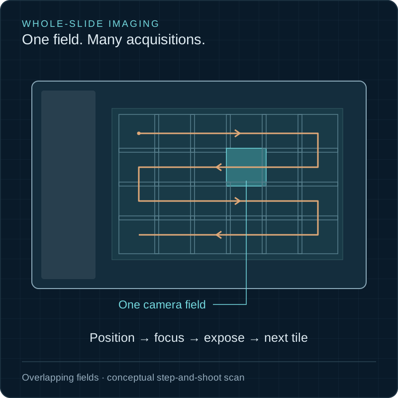
A scanner is one small field of view visited a few thousand times. Every specification that matters is really a question about what happens between two of those visits.
px ≤ 0.61λ / 2NA
Sampling is set by the objective, not by the sensor. The sensor and coupler only decide whether you meet it.
tiles ∝ 1 / px²
Halve the pixel size for finer detail and you quadruple the tiles, the scan time and the file. Nothing else in the machine has this exponent.
DOF ≈ λ / NA²
About one micron at NA 0.75 — across a slide that is not flat to within twenty. Focus, not resolution, is the hard problem.
Interactive throughput lab
Find out what is actually slowing the scan
Start from a workflow
Magnification at the sensor is the objective times whatever coupler follows it — a 20× objective behind a 0.5× tube adapter lands here as 10×.
Sampling
0.240 µm/px
Nyquist wants ≤ 0.336
Tiles per slide
232
1.31 × 0.88 mm each
Step-and-shoot
24 s
153 slides/hour
Uncompressed
11.7 GB
3.91 gigapixels
Where one tile's time goes
102 ms per tile, × 232 tiles
59% of every tile is the stage settling. The camera and the light are waiting on mechanics — a faster sensor buys you almost nothing here. Shorten the move, damp it better, or stop stopping: continuous scan finishes this slide in 10 s.
Resolution at λ = 550 nm, dry objective in air. Tile count assumes a rectangular raster over the quoted area; real tissue-finding trims it. Step-and-shoot charges one settle per tile and one frame period per channel; continuous scan charges frame periods only, and buys that with the flash duration below the bars.
This cameraStart here
A magnification number on a scanner tells you nothing
Scanners are sold as “20×” or “40×” instruments, and the number is close to meaningless on its own. Resolution comes from numerical aperture — an NA 0.5 objective resolves about 0.67 µm at green wavelengths no matter what magnification is printed on its barrel. Magnification only decides how that resolved detail is spread across pixels, and it is the objective and the coupler behind it that set the total.
So the first specification is not a magnification, it is a number in micrometres per pixel at the specimen. Sample coarser than half the resolvable separation and you are paying for an objective whose detail you then discard. Sample much finer and you have quadrupled the tile count, the scan time and the storage to record something the optics never delivered. Both mistakes are common, and both are invisible until someone multiplies out the arithmetic above.
Three ways to cover a slide
The architecture is a choice about stopping
Step-and-shoot
Area camera · simplest
Move, wait for the stage to settle, expose, read out, move again. Everything is deterministic and nothing needs to be synchronised. The settle time is charged once per tile, so throughput is a mechanics problem long before it is an optics one.
Continuous scan
Area camera · strobed
The stage never stops and a short flash freezes each frame. The settle time disappears from the budget entirely. In exchange the light must be gated in tens of microseconds and deliver a whole exposure inside that window.
Line scan and TDI
Line sensor · continuous
A line sensor sweeps the slide in continuous strips, so one axis has no tiles and no seams at all. TDI adds charge across stages to recover sensitivity at speed. It needs a uniform illumination line and a line rate locked to stage velocity.
The chain
Six subsystems, one shared clock
XY scanning stage
Carries the slide between tiles. Settle time, not top speed, is what you actually buy — a stage that moves in 20 ms and rings for 80 is a slow stage.
Motorised stagesZ focus actuator
Re-establishes focus at every tile against a depth of field near one micron. Repeatability and settle matter here; absolute accuracy does not.
Piezo Z stagesObjective and coupler
The objective sets NA and therefore resolution; the coupler that follows it sets magnification at the sensor. They are separate decisions and only the pair fixes your sampling.
Opto-mechanicsIllumination
Brightfield Köhler or fluorescence excitation. Switching speed, output stability over the length of a scan, and field flatness all end up in the image.
Specify a sourceEmission filtering
One filter set per channel. If channels are changed mechanically, the wheel is charged to every tile — the single largest hidden cost in multichannel scanning.
Optical filtersCamera
Sensor format is the throughput lever nobody quotes: doubling the tile area in both axes quarters the number of tiles you have to visit.
Scientific camerasThe hard problem
The slide is not flat and the tissue is not either
Depth of field at NA 0.75 is around one micron. A glass slide bows by tens of microns across its length, the coverslip adds its own tilt, the mounting medium varies in thickness, and the section itself is neither flat nor uniformly thick. The focal surface you actually need is a warped sheet several tens of microns deep, and you have a micron of latitude anywhere on it. Nothing else in a scanner is specified this tightly.
Two strategies exist and they fail differently. A focus map samples focus at a few dozen points first, fits a surface, then scans open-loop against it — fast, deterministic, and wrong wherever tissue thickness changes faster than the fit. On-the-fly autofocus measures at every tile, using a second sensor at a deliberate defocus or a short Z sweep, and survives folds, bubbles and torn sections at the cost of time or a second camera. Most instruments end up doing both: a map for the bulk, live correction where the map is not trusted.
What this asks of the hardware is worth stating precisely, because it is usually specified wrongly. Absolute Z accuracy is irrelevant — nobody cares what the true height is. What matters is repeatability and settle time: the actuator must land within a fraction of the depth of field and stop ringing before the exposure begins, a few thousand times per slide, without drifting over the hour. That is a closed-loop piezo specification, and it is the reason open-loop drive is not an option on the Z axis even where it is perfectly adequate in XY.
Illumination
The light is a specification, not a lamp
In a single-field microscope the illuminator only has to be bright enough and reasonably even. In a scanner it is charged to every tile, so its switching time, its stability and its uniformity are multiplied by several thousand before they reach the image. Five criteria, in the order they usually bite.
Switching, in microseconds and without a mechanism
A filter wheel or shutter costs 50–200 ms per channel change. On a four-channel scan of six hundred tiles that is twenty minutes of pure mechanism, and it wears. Per-channel electronic switching removes the line item rather than shrinking it.
Stability across the whole scan, not the first minute
A scan runs for minutes to an hour. Output drift over that period appears as a brightness gradient from one side of the slide to the other. Stitching cannot correct it, because the artefact is temporal and the correction is geometric.
Flatness across the full sensor field
Illumination non-uniformity becomes a visible grid once tiles are stitched — every tile carries the same shading, so the seams line up into a pattern the eye finds instantly. Flat-field correction removes the static part and nothing else.
Gateability at the flash duration continuous scan demands
Freezing motion to under one pixel at scanning velocity takes tens of microseconds. Delivering a full exposure inside that window is a peak-irradiance specification, and it is the reason brightfield goes continuous easily while fluorescence usually does not.
Bands matched to the fluorophores, with real out-of-band suppression
Excitation that bleeds into the emission band forces the filter set to do work the source should have done. In a scan that penalty is charged to every one of the tiles.
Detection
Sensor format is the throughput lever
E10ISPM20000KPA
20 MP across 5472 × 3648 at 2.4 µm. Behind a 0.5× coupler on a 20× objective it lands near 0.24 µm per pixel — the sampling most brightfield pathology is quoted at — and covers 1.3 mm of slide per tile.
- Sensor
- IMX383 (C,RS)
- Resolution
- 20M (5472×3648)
- Pixel Size
- 2.4 µm × 2.4 µm
- Frame Rate
- 49 fps @ 5472×3648(8-bit); 24 fps @ 5472×3648(12-bit); 49 fps @ 2736×1824(8-bit); 24 fps @ 2736×1824(12-bit); 120 fps @ 1824×1216(8-bit); 120 fps @ 1824×1216(12-bit)
sMAX04BM
Back-illuminated sCMOS at 72.5 fps. In fluorescence the exposure dominates the tile, so the value of a fast, low-noise sensor is that it takes readout out of the argument entirely.
- Sensor
- GSENSE2020BSI (sCMOS)
- Resolution
- 4.2 MP (2048×2048)
- Pixel Size
- 6.5 µm × 6.5 µm
- Frame Rate
- 72.5 fps @ 2048×2048; 72.5 fps @ 1024×1024
The detail that catches people out
A rolling shutter and a strobe do not automatically agree
Step-and-shoot under continuous illumination never raises this question, which is exactly why it ambushes people the first time they try to go faster. An sCMOS sensor with a rolling shutter starts and stops its rows in sequence, taking a fixed span to walk from the first row to the last. Fire a short flash at an arbitrary moment and it lands inside some rows' exposure windows and outside others: the frame comes back with a bright band across it, and no amount of flat-fielding removes it, because it moves.
The fix is to make an all-rows-open window exist and then put the flash inside it. That window only appears when the exposure is set longer than the row-readout span, so the last row has opened before the first one closes. Set exposure below that span and there is no instant at which the whole sensor is listening. The alternative is a global-shutter sensor, which sidesteps the geometry at some cost in noise or full-well.
Before you design a strobed continuous scan around a camera, confirm two things on its datasheet: that it publishes the row-readout span or line period, and that it accepts an external trigger with a deterministic delay. A camera that does neither can still scan — but only by stopping, which puts the settle time back into every tile.
Before you order
Six checks
- Fix the sampling in micrometres per pixel at the specimen, not in objective magnification. A “40× scanner” is undefined until the coupler is known.
- Measure the flatness of your own slides before committing to a focus strategy. If section thickness changes abruptly, a pre-computed focus map will fail exactly where the interesting tissue is.
- Specify the Z axis on repeatability and settle time. Absolute accuracy is not a requirement anywhere in this instrument.
- Compare settle against exposure before buying either. If settle is more than half the tile time, the money belongs in mechanics; if the exposure dominates, it belongs in light.
- Confirm the camera publishes its row-readout span and accepts an external trigger before designing around a strobe.
- Size storage and the sustained write path first. A gigapixel-scale scan that outruns the disk stalls the stage, and a stalled stage is a focus error.
Before you specify
Guides that cover this decision
 Scientific imaging
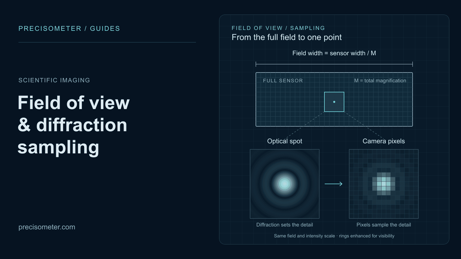
Calculating camera field of view and diffraction sampling
Calculate object-space pixel size, field of view, Rayleigh resolution, and sampling using real MAX and sMAX sensor formats.
Open guide Scientific cameras
How to select an sCMOS camera
Understand quantum efficiency, read noise, pixel size, SNR, and optical sampling using real MAX and sMAX specifications.
Open guide Motion control
Motorized linear stage selection
Why load capacity is really a moment specification, why Abbe error usually beats the quoted accuracy, why a rotary encoder on the motor is not position feedback, and when top speed is unreachable by geometry.
Open guide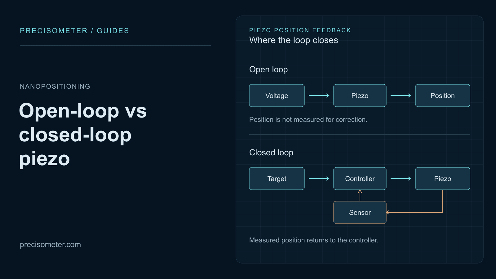 Nanopositioning
Open-loop vs closed-loop piezo
Why an open-loop piezo is wrong by 15 % of its travel, how creep grows with the logarithm of hold time, what strain-gauge and capacitive feedback actually fix — and the bandwidth and sensor noise a servo costs you in return.
Open guideSpecify the system
Tell us the tissue area, the sampling you need, and how many channels.
Those three numbers fix the tile count, and the tile count decides whether this is a mechanics problem or a photon problem.