Detect
Find a signal that differs reliably from the local background. Define the acceptable false-call and missed-defect behavior.
Semiconductor inspection · Selection guide
Choose what the instrument needs to detect, then connect the laser, collection optics, detector and scan timing. Build a source specification around the actual wafer and defect.
12 min guide · Interactive optical paths · Sampling and motion planner
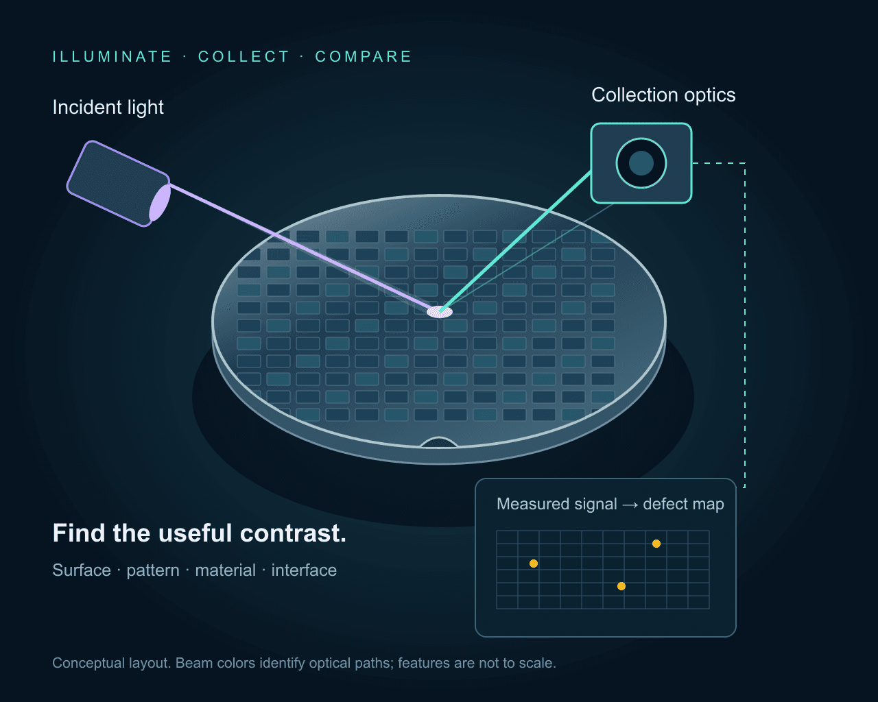
01 / Define the signal
Unpatterned wafers make surface contamination and background important starting points. A particle, scratch or film irregularity changes the returned optical signal. Scanning scatter measurements can use a point detector rather than forming a conventional camera image. Wavelength, incidence angle and collection aperture shape the result.
Patterned wafers add a strong, structured background. Image comparison needs registration, focus control and a suitable reference region. A repeatable difference can flag a process anomaly; identifying its cause may require higher-resolution review or another measurement. Treat electrical functionality as a separate verification.
Background: optical wafer-inspection methods and NIST’s treatment of collected scatter.
Scattered light
Particles, scratches and surface anomalies on bare wafers or films. Keep the strong specular reflection outside the collection path; collect light redirected by the sample.
Compare UV and visible excitation on the actual surface. Collection angle, polarization and film background matter alongside wavelength.
A bright scatter event is a detection signal. Its apparent image width is not the particle diameter.
Find a signal that differs reliably from the local background. Define the acceptable false-call and missed-defect behavior.
Separate nearby structures in the measured image. Wavelength, aperture, imaging mode and sampling all affect this capability.
Infer a dimension or defect class using a calibrated response or model. An intensity threshold alone is not a universal size measurement.
Subwavelength structures can influence a scattered-light signal even when their shape is not directly resolved. Extracting size or geometry then depends on a characterized optical system and a suitable model. NIST’s scatterfield work illustrates this distinction; it does not establish a sensitivity specification for the catalogue sources here.
02 / Select the excitation
Start with the material, film stack and defect response. Shorter wavelengths can change scattering, absorption and focus, but they also change the optical coatings, background and allowable dose. Compare candidates on representative wafers before setting the source architecture.
| Source class | Potential measurement | Selection check |
|---|---|---|
| CW UV · e.g. 266, 320 or 355 nm | Continuous surface scanning or material-specific excitation. | Measure contrast, sample response, UV transmission and power at the wafer. |
| Picosecond UV | Time-dependent excitation or a measurement that needs a defined pulse train. | Specify energy, duration, repetition rate and detection timing at one operating point. |
| Visible / violet CW | Reflected or scattered-light inspection with a suitable detector. | Compare polarization, speckle, beam profile and background on the target pattern. |
| Infrared / SWIR | Transmission or reflection through a suitable silicon path. | Measure the real stack transmission; match the detector and all optics to the band. |
The laser application overview provides the source-family starting points. For material-sensitive PL see surface and luminescence inspection methods. For buried silicon structures, continue with the SWIR semiconductor guide and infrared detector considerations.
CW illumination is a useful starting point for integrated-intensity measurements. Short pulses become relevant when the experiment needs time-resolved response or a short illumination interval. A camera integrating many pulses may still produce an intensity image; a picosecond pulse width alone does not create time resolution in the detector.
For a uniform pulse train, pulse energy is average power divided by repetition rate. As an illustrative calculation, 20 mW at 20 MHz gives 1 nJ per pulse. Focused intensity and cumulative dose still depend on spot size, pulse duration, scan overlap and dwell time. Heating, debonding and material removal require a separate process specification.
Long-term power stability and short-term intensity noise describe different behavior. Record averaging time, measurement bandwidth, warm-up and ambient conditions. Pointing drift can change the illuminated location or the signal admitted by a collection aperture, even if total laser power is stable.
Also define polarization, beam diameter, divergence, profile and delivered power after conditioning optics. Narrow linewidth is valuable when the measurement needs it; coherent speckle can complicate intensity comparison. Qualify any homogenizer, line generator or fiber delivery at the required wavelength and dose.
03 / Connect motion and acquisition
Use the planner for an imaging or line-scan configuration. The sensor pitch and total magnification set the object-plane sample spacing. Scan speed and effective exposure set the motion accumulated during one measurement. These are geometry calculations, not a defect-sensitivity prediction.
Assumes constant linear motion, a fixed magnification and a rectangular effective exposure. For a scanning beam, use the local spot velocity; a rotating wafer has a radius-dependent speed.
Motion stays within the example 0.5 px budget.
The 0.5 px budget is a planning choice. Shorter exposure reduces motion but also reduces detected signal unless the illumination changes. Verify the camera line rate, readout and trigger behavior separately.
Sampling = pixel pitch / magnification. Motion = speed × exposure. Line rate = speed / sampling, for one sample spacing per line; this is not an area-camera frame rate. No readout, overlap, acceleration or data-transfer overhead is included.
These values do not predict optical resolution, signal-to-noise ratio or a minimum detectable defect size.
A 5 µm sensor pixel at 10× magnification samples 0.5 µm at the wafer. At 5 mm/s and 50 µs effective exposure, translation is 0.25 µm, or 0.5 pixel. A line scanner advancing by one sample spacing per line would need a nominal 10 kHz line rate. The optical image, collection efficiency and detector noise still determine whether a defect is detectable.
Check exposure outputs, encoder triggers, latency, jitter and data-transfer limits for the exact acquisition mode. TDI acquisition requires motion and signal transfer to stay synchronized. For a rotating wafer, local tangential speed changes with radius, so a single linear-speed example is not a whole-wafer scan recipe. Read the TDI synchronization background.
04 / Precisometer source examples
These existing catalogue examples illustrate different excitation architectures. Their model sheets govern power, stability, pulse duration and repetition rate. Match delivered power and dose to the sample; the highest catalogue power is not an inspection requirement.
CW UV · 266 nm
Evaluate UV surface contrast or material-specific excitation; confirm UV optics and delivered dose.
CW UV · 320 nm
An excitation option when the sample response and collection filters favor this UV line.
CW UV · 355 nm
Compare continuous UV excitation for scanning or luminescence measurements on the actual material.
Picosecond UV · 266 nm
Consider when the measurement requires short-pulse excitation. Specify pulse energy, timing and sample dose together.
Picosecond UV · 355 nm
A pulsed UV alternative for a timing-dependent experiment; verify its operating point against the model sheet.
Visible / violet CW · 405 nm
Evaluate reflected or scattered-light contrast with a matching camera, illumination profile and power control.
Infrared CW · 1550 nm
A candidate for a transmitting silicon path, with an infrared-sensitive detector and verified optical transmission.
05 / Establish acceptance evidence
Include the real substrate, films, pattern and process stage. Record known defect locations and independent review results. Reference particles help characterize a response; they do not automatically represent every real contaminant or crystal defect.
Capture dark and reference signals, correct illumination nonuniformity where appropriate, and check saturation. Verify delivered power and revisit the same locations to look for exposure-induced change. Keep the illumination recipe with the data.
Repeat scans after repositioning and across the useful field. Vary focus and scan direction to identify geometry-dependent artifacts. Check whether apparent defect contrast follows the wafer, the illumination path or the acquisition timing.
Evaluate true detections, missed defects and nuisance calls on the reference set. Record recipe settings and uncertainty, and separate automated screening from subsequent defect review. Throughput must include alignment, handling, acquisition, processing and review.
Include material and layer stack, patterned or bare surface, defect classes and reference samples, excitation and detection bands, allowed dose, field of view, scan speed and acceptance criteria. Define the required source, delivery, detector, motion and software scope together.
Build an inspection enquiryPractical answers
No. Wavelength changes the interaction and the optical response, but detection also depends on defect material, shape, the wafer stack, collection geometry, background and detector noise. A scatter signal from a subwavelength object does not mean the system resolves its shape or measures its size directly.
CW illumination can suit steady scanning and integrated-intensity measurements. Use picosecond excitation when timing, time-resolved emission or another defined measurement requires it. Average power alone does not specify pulse energy or peak intensity, and short pulses do not guarantee a non-damaging inspection dose.
The same source may be useful in different experiments, but the excitation response, emitted spectrum, surface reflection and acceptable dose can differ. Qualify wavelength, collection filters and detector for each material and defect class.
No. It calculates object-plane sampling, translation during exposure and a nominal line-scan rate from the entered geometry and speed. It does not model diffraction, scattering strength, signal-to-noise ratio or a minimum detectable defect size.
The linked catalogue contains laser sources, detectors, cameras, optics and positioning components for integration. The supply scope, wafer handling, cleanliness, autofocus, processing software and acceptance criteria must be defined for the proposed system.
The overview introduces the source families; the independent technical references explain measurement principles. Product-specific limits belong to the linked model datasheets. The diagrams and planner are educational, with no claimed wafer-level detection limit.
Before you specify
 Semiconductor inspection
Design a through-silicon inspection setup for wafers and ICs: choose transmission, reflection, or emission imaging; then match wavelength, NA, sampling, and camera.
Open guide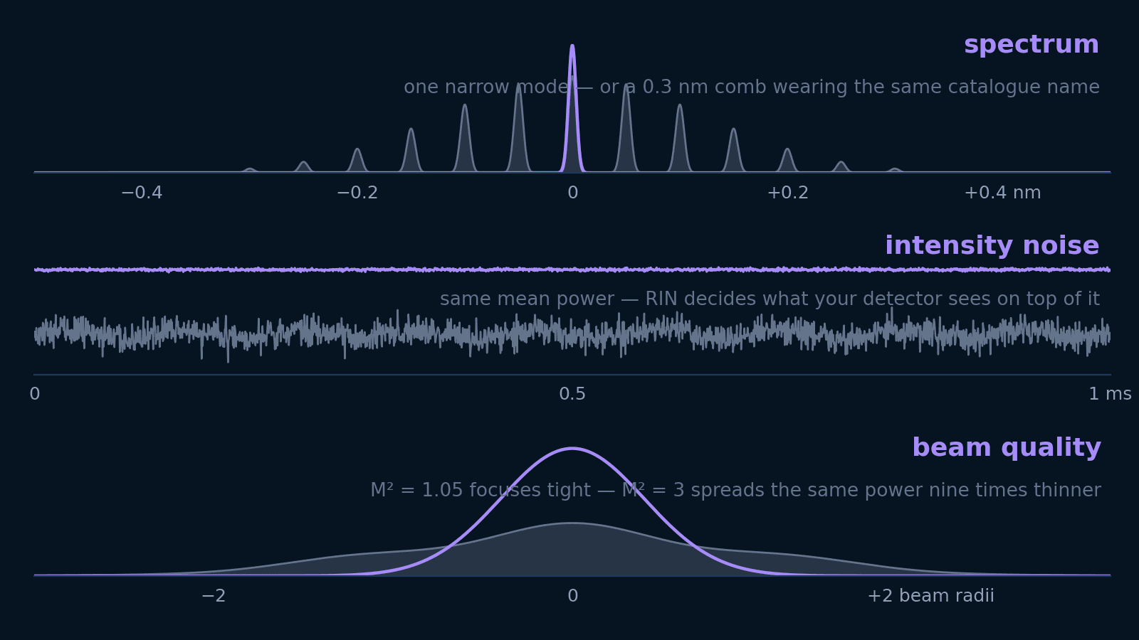 Photonics
Linewidth, spectral width, RIN, M², and coherence length answer five different questions. Translate each into the units your experiment is designed in — and learn which ones not to pay for.
Open guide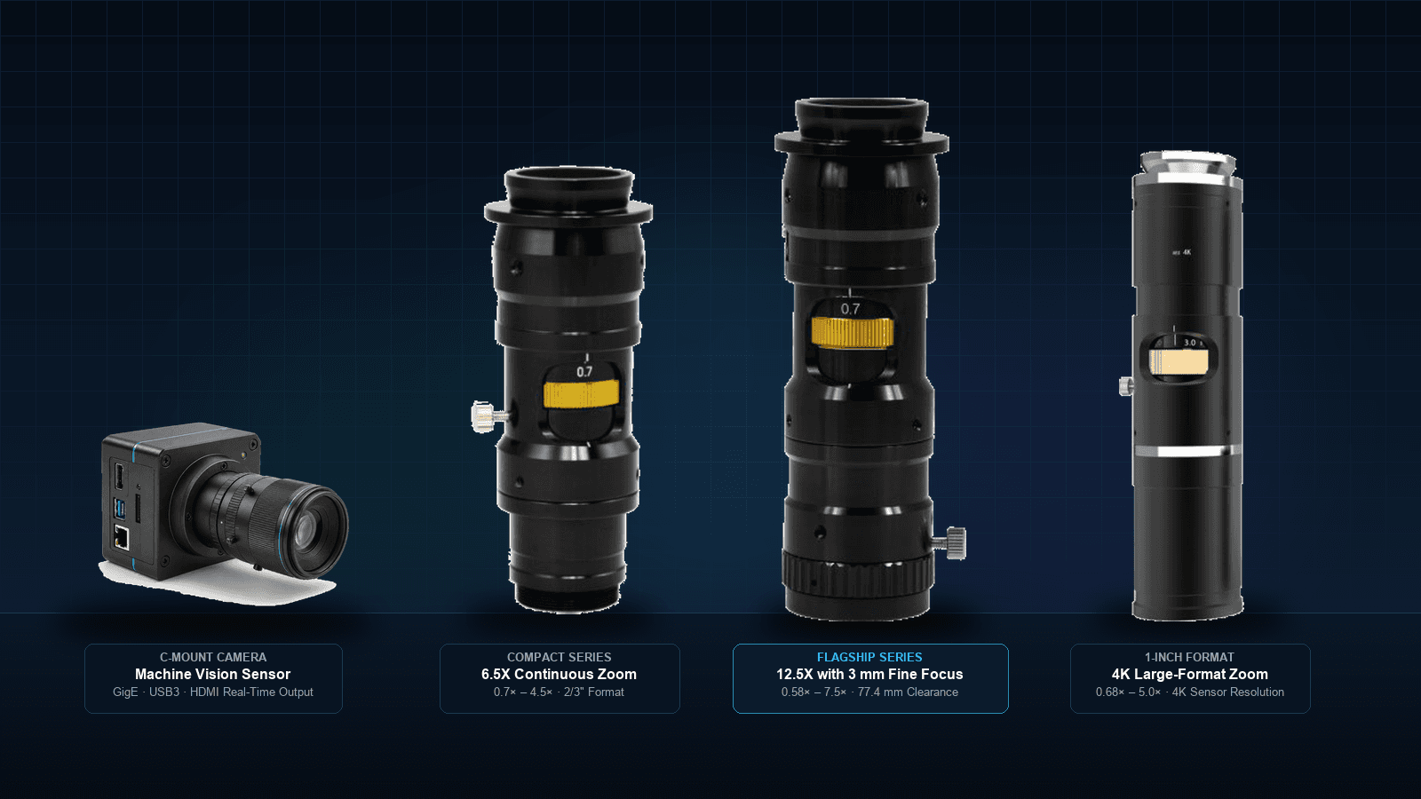 Machine vision
Turn a part, defect size and working distance into a magnification, camera and specific zoom-lens version. Includes the interactive Inspection Optics Planner to test FOV, Rayleigh resolution and depth of field.
Open guide