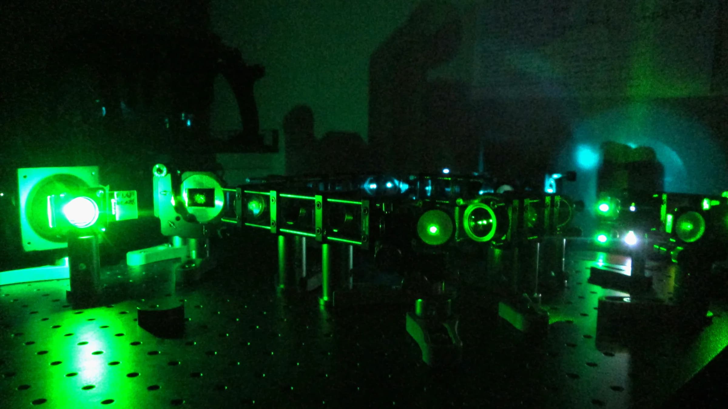
Optics laboratory, UCL Department of Physics & Astronomy, London · Photo: Isabel Llorente Garcia / UCL MAPS · CC BY 2.0
Complete experiment guide
Building a pump–probe spectroscopy system
Design the pump, probe, delay line, monochromator, camera, and timing chain as one instrument—from femtosecond overlap to the final transient spectrum.
Pump creates the clock
A short pulse prepares a non-equilibrium state at a defined fluence and wavelength.
Delay becomes the time axis
A controlled path difference determines when the probe interrogates that state.
Detection defines the observable
Photodiode, camera, and monochromator decide whether you record one kinetic trace, a spectrum, or an image.
The decision in one sentence
Choose the dynamics and observable before choosing the hardware.
Pump–probe spectroscopy is a differential measurement. The useful signal is often many orders of magnitude smaller than the probe itself, so temporal resolution, wavelength coverage, detector bandwidth, dynamic range, and reference strategy cannot be optimized independently.
Name the process
Electronic relaxation, charge transfer, vibrational cooling, phase change, carrier transport, or heat.
Bound the axes
Earliest resolvable time, longest delay, pump wavelength, and probe spectral region.
Define the smallest signal
Expected ΔA or ΔR/R, sample damage threshold, and time available per delay point.
1 · Signal + sign
Measure the probe twice, then take the difference.
1 · Excite
The pump prepares a small fraction of the sample at a controlled fluence and polarization.
2 · Wait
Optical path or electronic timing sets the pump-to-probe delay.
3 · Interrogate
The probe records transmission, reflection, polarization, emission, or another response.
4 · Normalize
Pump-on and pump-off measurements are paired, referenced, and repeated across delay.
Transient absorbance
The sign labels mechanisms, not certainty. Spectral overlap, stimulated emission, scattering, coherent artifacts, and thermal signals can coexist at the same pixel.
A kinetic trace is not automatically one population.
A fixed probe wavelength can sit on a shifting or narrowing band, a bleach, and an induced absorption at once. Broadband spectra and global analysis help separate correlated spectral evolution from true population decay.
2 · Measurement architecture
One timing principle, several observables.
The detector architecture should follow the information you need—not a generic definition of pump–probe.
Broadband transient absorption
- Probe
- White-light continuum or another broadband pulse
- Detector
- Spectrograph plus line or area array
- Best for
- A two-dimensional map of wavelength versus delay
Tradeoff: Maximum information per delay, with chirp correction and demanding shot-to-shot normalization.
Single-color pump–probe
- Probe
- Narrowband pulse at one diagnostic wavelength
- Detector
- Photodiode and lock-in or boxcar detection
- Best for
- Fast, sensitive kinetics at a known spectral feature
Tradeoff: Simpler and often more sensitive, but spectral evolution can masquerade as population dynamics.
Pump–probe microscopy
- Probe
- Focused probe scanned across the specimen
- Detector
- Photodiode, balanced detector, or synchronized camera
- Best for
- Spatially heterogeneous carrier, thermal, or structural dynamics
Tradeoff: Adds focus overlap, image registration, dwell, and dose to the temporal measurement.
Complete path
The reference channel belongs inside the architecture.
Laser
Shared timing origin
Split + gate
Pump / probe + AOM
Delay
Retroreflector or clock
Sample
Spatial + temporal overlap
Filter
Reject residual pump
Disperse
Monochromator / spectrograph
Detect
Signal + optional reference
3 · Pulses + delay
The stage does not set time resolution by itself.
Pulse duration, chirp, jitter, crossing geometry, wavelength-dependent group delay, and the sample response all broaden the effective instrument function.
Pulse duration
The pump and probe widths set the best possible cross-correlation before jitter, chirp, geometry, or sample response are included.
Time zero
Measure temporal overlap with a suitable nonlinear or instantaneous response; the mechanical zero of the stage is not the optical zero.
Delay window
A retroreflector doubles optical path: 1 mm of stage travel changes delay by about 6.67 ps.
Delay sampling
Use finer steps around time zero and early dynamics; logarithmic or segmented spacing is usually more efficient at long delays.
Repetition period
The sample should substantially recover before the next pump pulse unless steady-state accumulation is part of the model.
Clock ownership
Laser, pump modulator, stage, camera or digitizer, and reference channel must agree on shot identity.
Gaussian starting estimate
τcc ≈ √(τpump² + τprobe²)
Useful for transform-limited Gaussian pulses. Add measured jitter and other independent broadening terms in quadrature only as a first engineering model.
Retroreflector delay
Δt = 2Δx / c
A 1 µm stage move gives about 6.67 fs of delay; 150 mm gives about 1 ns. Resolution, travel, straightness, settling, and encoder accuracy are separate specifications.
Use a pulse picker to change shot identity—not pulse duration.
An AOM diffracts selected pump pulses into the experiment so the effective repetition rate or pump-on/off pattern can be synchronized to the detector. It does not make the femtosecond pulse shorter. The RF gate must be phase-locked to the laser, and the acoustic rise time, diffraction efficiency, extinction, dispersion and peak-fluence limit all belong in the timing budget.
Important: broadband chirped probes can have a sample-dependent effective temporal response. A single cross-correlation number does not guarantee the same resolution at every wavelength or for every kinetic model.
4 · Probe + monochromator
Convert a continuum into calibrated detector pixels.
The spectrograph decides how much wavelength lands on each pixel and how much light reaches it. Focal length, grating, slit, detector width, and input f/number are one coupled choice.
Spectral span
Coverage per frame is reciprocal linear dispersion multiplied by active sensor width.
Bandpass
The slit image, aberrations, and detector pixels combine into the recorded width of a narrow feature.
Throughput
A narrower slit and slower f/number reduce photons per spectral bin, often before resolution becomes useful.
Track geometry
Signal and reference spectra need focal-plane height, low astigmatism, and enough pixel rows to remain separate.
Survey spectrum
Low groove density · wide slit
Maximize wavelength span and photons while locating broad transient features.
Balanced kinetics
320 mm class · moderate slit
Resolve evolving bands without starving every camera pixel.
Narrow transient line
Higher dispersion · narrow slit
Use only when a known feature actually requires the extra bandpass.
5 · Cameras + detectors
Match detector material and readout to the probe.
A camera is useful only if its active width captures the required spectrum, its pixels sample the bandpass, and its trigger/readout pattern preserves pump-on versus pump-off shot identity.
UV–visible
Back-illuminated silicon CCD or sCMOS
High quantum efficiency, fine pixels, mature low-noise arrays
Verify UV coating or window, rolling/global timing, full well, and the QE curve at every probe wavelength.
Visible–NIR
Silicon array to roughly the silicon cutoff
One detector can cover common white-light continua through much of the visible and near-IR
Sensitivity can fall steeply near the long-wavelength edge even when the nominal range still includes it.
SWIR · 900–1700 nm
InGaAs line or area array
Direct broadband detection beyond silicon with high-speed line-scan options
Pixel pitch, cooling, read noise, well depth, detector nonlinearity, and Camera Link bandwidth become central.
Single wavelength
Si, InGaAs, or other matched photodiode
High electrical bandwidth and straightforward lock-in or balanced detection
Choose bandwidth from the modulation frequency and pulse integration scheme—not the femtosecond pulse width itself.
Line-scan array
Best detector geometry for one spectrum at high rate; every pixel can map to wavelength.
Area camera
Supports reference/sample tracks, imaging spectra, or spatially resolved pump–probe—but reads more data.
Photodiode
Best when one wavelength and high modulation sensitivity answer the question.
Frame rate is a system property. Full-frame fps, ROI or line rate, exposure, interface bandwidth, trigger latency, dead time, and chopper pattern together determine whether adjacent pump-on/off pulses can be paired. Never infer shot-to-shot capability from a headline frame rate alone.
6 · System calculator
Place timing and spectral detection on the same budget.
The instrument response, stage window, repetition period, spectrograph coverage, camera sampling, and acquisition clock constrain one another. Use the lab to expose mismatches before hardware selection.
Model the instrument
Pump–probe design lab
Illustrative configurations; each preset updates the full timing and detection chain.
Calculated system envelope
The increment is 6.67 fs; a useful first-pass target is no more than half the 159 fs instrument response.
The pulse period is 1,000,000 ns, or 1,000× the selected recovery time. Verify this experimentally through repetition-rate and fluence scaling.
The timing model assumes Gaussian pump and probe pulses, an independent FWHM-equivalent jitter contribution, and a retroreflector giving twice the stage displacement as optical path. The spectral estimate combines slit width, a nominal 30 µm aberration blur, and 2.5-pixel sampling in quadrature. Acquisition time is an ideal photon-clock minimum: camera rate, chopper, readout, stage settling, references, and repeats can dominate.
7 · Noise + artifacts
Design controls into the experiment—not just into analysis.
The most convincing pump–probe result survives changes in fluence, polarization, repetition rate, sample position, delay order, and detection scheme.
Coherent artifact
Pump and probe overlap can create cross-phase modulation, two-photon absorption, or interference near time zero.
Change polarization, pump fluence, crossing geometry, solvent or substrate, and compare against an unexcited reference.
White-light chirp
Different probe wavelengths arrive at different times after continuum generation and dispersive optics.
Measure wavelength-dependent time zero and correct it before interpreting spectral motion as kinetics.
Pump scatter
Residual pump light can reach the detector and inherit the pump modulation exactly.
Use spatial separation, spectral filters, beam dumps, polarization, and background measurements without the probe.
Accumulation
Long-lived states or heating survive until the next pump pulse.
Reduce repetition rate, translate or flow the sample, and test the signal against pulse energy and repetition independently.
Nonlinear regime
A nominally first-order transient changes shape or lifetime with pump fluence.
Build a fluence series and select the lowest regime that still meets the required signal-to-noise ratio.
Probe instability
Continuum structure and intensity fluctuate much more than a narrowband laser.
Record pump-on/off pairs shot to shot and add a simultaneous reference spectrum when the noise budget justifies it.
Laser clock
Defines every pulse.
Pump modulator
Assigns on/off identity.
Detector trigger
Captures the correct pulse or pulse group.
Stage encoder
Attaches calibrated delay to every record.
8 · Relevant products
Build the instrument stack from the measurement outward.
These catalog-backed starting points cover ultrafast excitation, optical delay, pulse selection, beam routing, visible and SWIR detection, and two spectrograph geometries. They are not automatic system matches; interfaces and clocks still need a joint review.
Timing, pulse selection and delay
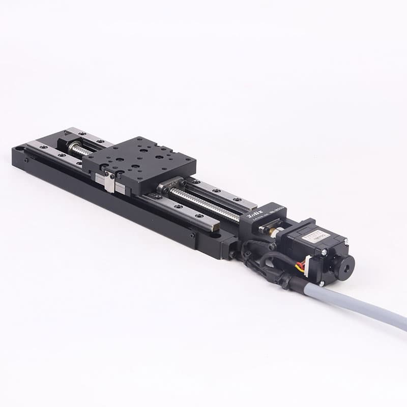
LA150-60
The long-travel LA platform is a practical starting point for a retroreflector delay arm when the experiment needs hundreds of picoseconds through roughly one nanosecond of mechanical delay.
- Mechanical travel
- 150 mm
- Double-pass delay window
- ≈ 1.00 ns
- Minimum incremental motion
- ≤ 2 µm · ≈ 13.3 fs
- Micro-step repositioning
- ≤ ±1 µm
- Maximum speed
- 20 mm/s
Qualify: The stage is the moving platform, not the complete optical delay. Add a low-dispersion roof-mirror or corner-cube assembly, compatible controller, beam enclosure and home/limit strategy. Validate settling, approach direction and actual optical repeatability in the assembled interferometric geometry.
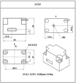
AOM-I acousto-optic modulator
An AOM can assign pump-on and pump-off shots, reduce the effective repetition rate, or create a synchronized modulation pattern before the sample.
- 450–700 nm
- 100 MHz centre frequency
- Up to 4 MHz pulse repetition
- 80% diffraction efficiency
- TTL / analogue control
Ultrafast check: The catalog AOM-I is specified for typical optical power below 1 W with a 1.0 mm beam. Before using it with femtosecond pulses, confirm wavelength, single-pulse energy, beam diameter, peak fluence, dispersion, extinction, thermal load, acoustic rise time and RF-driver timing with the supplier.
Zolix beam-routing optomechanics
Use stable mounts and a consistent beam height around the delay arm. The final retroreflector geometry, mirror coatings and apertures must match the pump or probe wavelength and beam diameter.
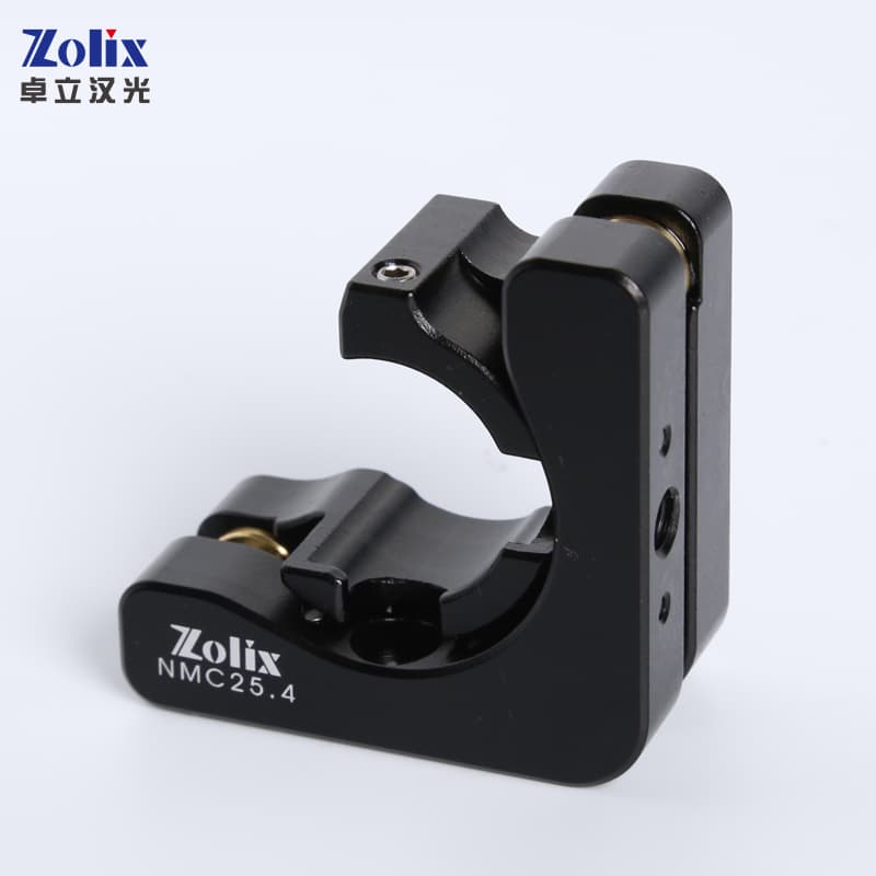
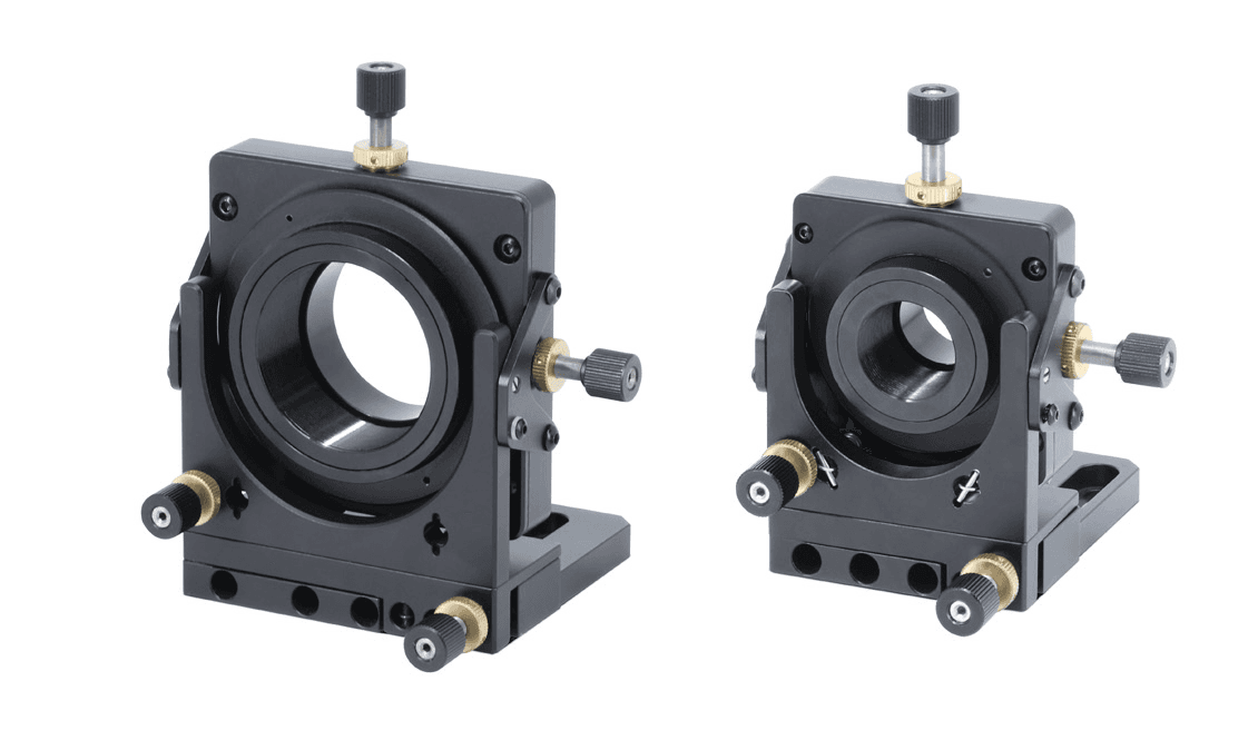
NMC25.4
Centre kinematic mount for Ø25–25.4 mm optics, useful for steering the pump and probe while keeping the mirror centre easy to reference.
- ±3° angular range
- Ø23 mm clear aperture
- 25 mm optical-axis height
NMUM25.4
Five-axis mount for positioning a 25.4 mm optic where beam position, focus and angle must all converge at the sample.
- ±2.5 mm X/Y
- 6 mm Z travel
- ±5° tip/tilt
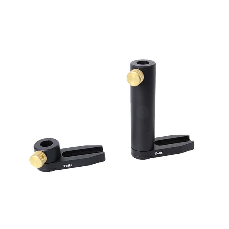
NPH50
A compact base-mounted holder for Ø12 mm posts that helps keep delay-line and steering optics at a repeatable table height.
- Ø12 mm post
- 50 mm overall height
- Base-mounted holder
Ultrafast laser starting points
FS-F-1030A
A 1030 nm femtosecond source family for experiments that use the fundamental for probe-continuum generation and derive pump wavelengths through harmonic or parametric conversion.
- Output / average power
- 1-10 W
- Repetition rate
- 1 MHz
Qualify: Confirm pulse width at the experiment, pulse energy after splitting, continuum stability, trigger outputs, and whether the sample fully recovers at 1 MHz.
FS-F-515B
A 515 nm femtosecond source with a 100 kHz–1 MHz catalog repetition range for direct green excitation or a synchronized branch of a wider ultrafast platform.
- Output / average power
- 2-8 W
- Repetition rate
- 100 kHz-1 MHz
Qualify: Size fluence at the sample and verify the chosen repetition rate against the longest-lived state, heating, and detector acquisition strategy.
Monochromators and spectrographs
HiperS-320i
An aberration-corrected focal plane is valuable when probe and reference spectra occupy separate detector tracks or when a fiber bundle must remain spatially resolved.
- 320 mm focal length
- f/4.4 aperture
- 2.29 nm/mm dispersion*
- 29 × 14 mm focal plane
Qualify: Choose grating, blaze, slit image, input f/number, detector format, and pump-rejection filtering as one optical design.
Omni-λ300i
A practical 320 mm Czerny–Turner platform when moderate spectral resolution, throughput, and a configurable triple-grating turret must coexist.
- 320 mm focal length
- f/4.2 aperture
- 2.3 nm/mm dispersion*
- 30 × 14 mm focal plane
Qualify: Calculate the wavelength span on the actual sensor and avoid paying for resolution that only reduces photons per pixel.
Scientific cameras and arrays
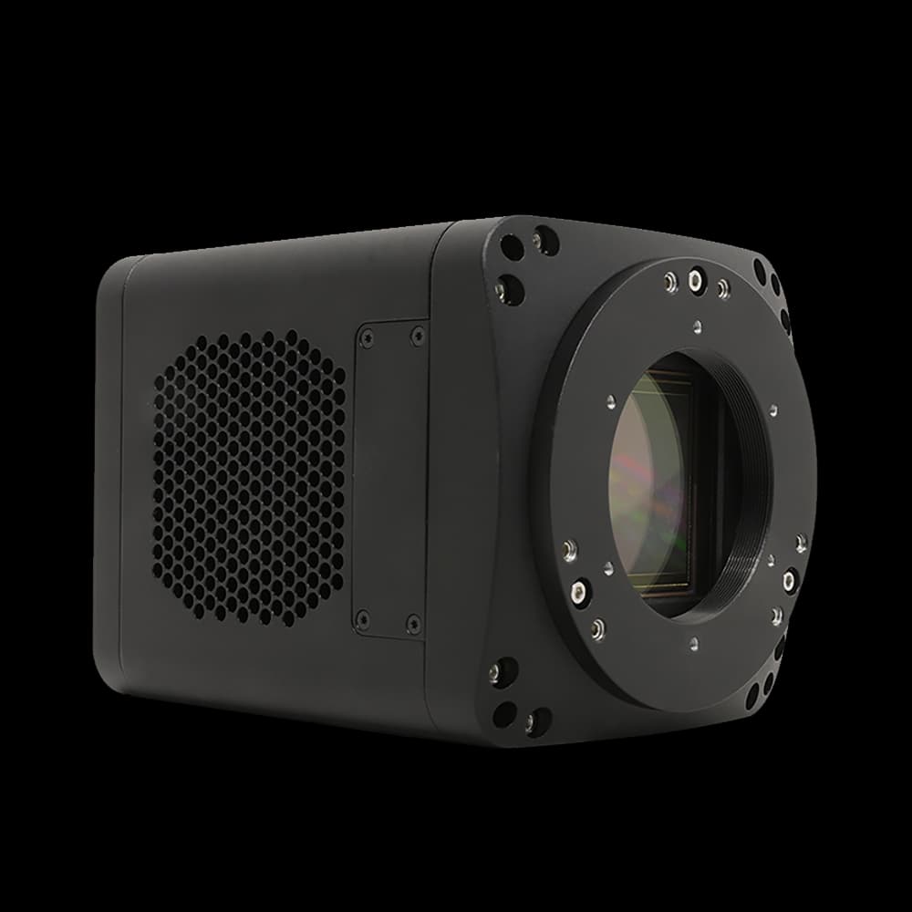
sMAX04BM-CL100
A 2048 × 2048 back-illuminated scientific sCMOS format with Camera Link and 108 fps full-frame readout for spectrally and spatially resolved acquisition.
- Sensor
- GSENSE2020BSI (sCMOS)
- Resolution
- 4.2 MP (2048×2048)
- Pixel Size
- 6.5 µm × 6.5 µm
- Frame Rate
- 108 fps @ 2048×2048; 108 fps @ 1024×1024
- Interface
- Camera Link
Qualify: Full-frame rate is not the same as laser-shot rate. Verify ROI timing, external trigger behavior, global-reset sequence, read noise, well depth, and pump-on/off pairing.
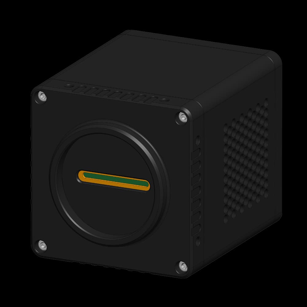
SWIR2048L3A-CL80K
A 2048-pixel InGaAs line-scan detector spanning 900–1700 nm with a 79 kHz catalog line rate and 25.6 mm active length.
- Sensor
- China-made 2048-pixel line-scan sensor
- Resolution
- 2048 pixels (2048 × 1)
- Pixel Size
- 12.5 µm × 12.5 µm
- Frame Rate
- 79K @ 2048 × 1
- Interface
- CameraLink Full
Qualify: Match the Camera Link acquisition clock to the laser and chopper, and verify that 12.5 µm pixels correctly sample the chosen monochromator bandpass.
Need the complete pump–probe chain reviewed?
Bring the process timescale, pump wavelength and fluence, probe band, target ΔA, sample recovery time, delay window, and preferred acquisition rate.
*Dispersion values shown for the catalog reference grating and wavelength; actual dispersion changes with grating, wavelength, and geometry.
9 · Specification brief
Specify a measurement, not a shopping list.
These inputs expose the interfaces between the laser, mechanics, spectroscopy, detector, and software before procurement.
Observable
Transmission, reflection, polarization, emission, or an image; expected ΔA or fractional-signal range.
Pump
Wavelength, pulse width, energy at sample, spot size, fluence, polarization, repetition rate, and modulation.
Probe
Single wavelength or continuum, spectral range, pulse width, chirp, spot size, polarization, and reference split.
Delay
Required negative delay, maximum positive delay, step near time zero, repeatability, and continuous or stepped scan.
Sample
Thickness, substrate or solvent, damage threshold, longest recovery time, motion or flow, and environmental control.
Spectrograph
Wavelength span per frame, target bandpass, grating and blaze, slit width, input f/number, ports, and stray-light needs.
Detector
Material, QE curve, pixel pitch, active width, read noise, full well, bit depth, cooling, frame or line rate, and trigger latency.
Acquisition
Pump-on/off pattern, shot identity, reference channel, averages, delay order, metadata, and calibration schedule.
10 · Common questions
Short answers before the design review.
What does pump–probe spectroscopy measure?+
It measures how a probe signal changes after an earlier pump pulse perturbs the sample. Repeating that measurement versus delay reconstructs excited-state, carrier, vibrational, structural, or thermal dynamics within the observable selected by the probe.
Is transient absorption the same as pump–probe spectroscopy?+
Transient absorption is one major pump–probe implementation: the observable is the pump-induced change in optical density across one or many probe wavelengths. Pump–probe also includes transient reflectance, Kerr signals, microscopy, photoemission, diffraction, and other observables.
How long a delay can a translation stage provide?+
With a retroreflector, the delay is approximately 6.67 ps per millimetre of stage travel. A 150 mm stage therefore provides about 1 ns of optical delay. Longer windows usually need electronic timing, pulse picking, a second source, or asynchronous sampling.
Should I use a camera or a photodiode?+
Use an array when the spectrum itself changes and must be captured at once. Use a photodiode when one wavelength is sufficient and sensitivity or modulation bandwidth matters more than spectral coverage. A camera does not automatically provide shot-to-shot detection: its trigger and readout must match the laser and chopper.
How much spectral resolution is enough?+
Enough to distinguish the narrowest transient feature that matters, sampled by at least a few detector pixels. Broad electronic bands often benefit more from photons and wavelength coverage than from a long focal length or a very narrow slit.
Why use a reference spectrum?+
A simultaneous reference channel can remove common probe fluctuations when signal and reference experience the same continuum noise. It cannot correct pump scatter, sample motion, detector nonlinearity, or different optical transfer functions between the two tracks.
Research basis
This guide is an engineering overview. Representative primary studies supporting the timing, cross-correlation, broadband detection, and acquisition discussions include:
- 1. Polli et al., “Effective temporal resolution in pump-probe spectroscopy with strongly chirped pulses,” Physical Review A 82, 053809 (2010).
- 2. Rasmusson et al., “On the use of two-photon absorption for determination of femtosecond pump–probe cross-correlation functions,” Chemical Physics Letters 335, 201–208 (2001).
- 3. Kanal et al., “100-kHz shot-to-shot broadband data acquisition for high-repetition-rate pump-probe spectroscopy,” Optics Express 22, 16965–16975 (2014).
- 4. Schmidhammer et al., “A broadband ultrafast transient absorption spectrometer covering the range from near-infrared down to green,” Applied Spectroscopy 68 (2014).
- 5. Domke et al., “Ultrafast pump-probe microscopy with high temporal dynamic range,” Optics Express 20, 10330–10338 (2012).
Continue designing