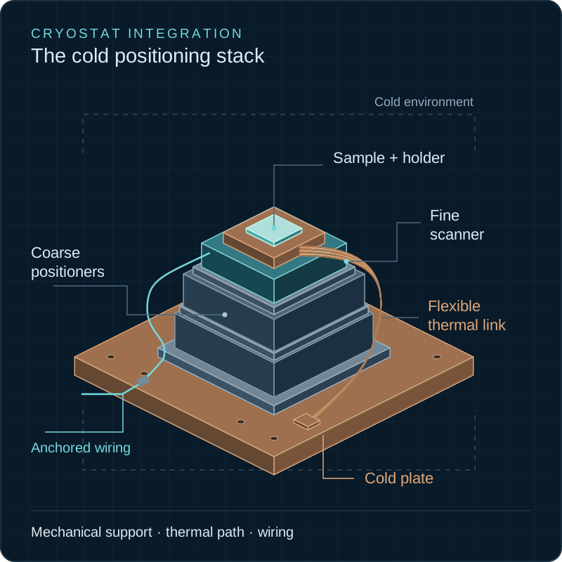
01 · Start with the experiment
The cryostat writes the specification. The stage only has to meet it.
A positioning system inside a cryostat is constrained from the outside in. The cold plate fixes the temperature and how much heat you may add to it; the shields fix the envelope; the magnet fixes what materials are allowed and which directions carry torque; the wiring loom fixes how many lines you get and what waveform they can carry. Only after those are written down does travel, resolution or payload become a choice rather than a consequence.
Two of these constraints are routinely misread. The first is temperature: the base temperature of the cryostat is the temperature of its coldest plate with nothing on it, and the sample on top of a stack of titanium stages is not at that temperature unless you build the path that makes it so. The second is cooling power: a 4 K plate under a pulse tube has of the order of a watt to spare, so stepping heat is a nuisance; the mixing chamber of a dilution refrigerator has tens of microwatts at 20 mK and a few hundred at 100 mK, so the same stepping is the dominant load and has to be scheduled.
Our selection guide covers the six gates that decide the model family. The worksheet below is the integration version: the numbers we need from you to turn a family into a stack that fits your cryostat, and the reason each one matters.
| Requirement | What to write down | What it decides |
|---|---|---|
| Base temperature | Cold-plate temperature with the stage installed, not the empty-cryostat figure. | Sets the .ULT option (30 mK) versus the standard 1.4 K grade, the body material, and how much heat the stack may add. |
| Sample temperature | What the measurement needs at the sample, and how long it must stay there. | Decides how much thermal path you must build: braid length, interfaces, sensor excitation policy. |
| Cooling power at the plate | Available cooling power at the plate the stack mounts to, at the temperature you will run at. | A 4 K plate offers watts; a mixing chamber offers microwatts. The same stepping duty cycle is invisible on one and dominant on the other. |
| Pressure and bakeout | Exchange gas, HV (~10⁻⁷ mbar) or UHV (~10⁻¹¹ mbar); bakeout temperature and duration if any. | Selects the .HV (default) or .UHV grade and the connector materials; the published operating range tops out at 400 K. |
| Magnetic field | Magnitude, direction relative to each motion axis, and whether the field ramps during motion. | All series are rated to 35 T, but torque on a magnetic sample and eddy damping in moving conductors are your problem to bound. |
| Payload and moment | Mass, size and centre-of-gravity height of everything the bottom stage carries, including upper stages and cables. | Compared against per-model load ratings (50 g to 2.5 kg) and against stack stiffness. |
| Envelope and mounting | Free volume, bore diameter, mounting hole pattern and material of the plate. | Chooses the 16, 25 or 35 mm series, the installation plate, and whether a vertical adapter is needed. |
| Optical or probe access | Direction of access, working distance, clear aperture through the stack. | Optic variants with a through-aperture; stack height versus objective working distance at base temperature. |
| Travel | Coarse travel per axis (mm or degrees) and fine scan range at operating temperature. | Coarse travel is mechanical and survives cooldown; fine range shrinks with temperature and is quoted separately at 4 K. |
| Resolution, repeatability, stability | Smallest useful move, return-to-position tolerance, and hold tolerance over the measurement time. | Open-loop versus resistive versus capacitive feedback; whether a closed-loop Ultra scanner is justified. |
| Duty cycle | Moves per hour, steps per move, hold time between moves. | Stepping heat versus quiescent heat; whether coarse motion can be scheduled away from the measurement window. |
| Wiring and interface | Lines available on the loom, feedthrough type, controller interface and trigger needs. | Channel count, controller choice, whether the fridge loom can carry a 200 V sawtooth at all. |
Fill the worksheet into our contact form and we will return a stack, controller and accessory list against it. The form opens pre-filled with these twelve lines.
Request a configuration with this worksheetResolution
The smallest position change the system can produce or detect. A sub-nanometre fine-tune step says nothing about where the stage is in absolute terms.
Accuracy
How close a commanded position is to the true position. Needs a calibrated sensor: resistive encoders on coarse stages resolve ~150 nm, and their scale shifts with temperature, so accuracy exists only after calibration at the operating point.
Repeatability
How closely the stage returns to the same position on repeated commands. Coarse stages: 1–2 µm; Ultra scanners: < 5 nm in the manufacturer test at 4.2 K.
Stability
How far the position wanders while nothing is commanded, over the measurement time. Set by creep, thermal drift and vibration, not by the actuator resolution.
These four are different quantities, and a datasheet resolution figure is the least informative of them. State which one the experiment actually needs, over what time.
02 · Choose coarse positioning and fine scanning
Two mechanisms, because no single actuator covers millimetres and nanometres cold.
A stick-slip stage moves by a sawtooth: a slow flank drags the slider with the piezo, a fast flank lets it slip back. Travel is set by the guide, not by the ceramic, so the 3–20 mm of a Linear stage or the 30–200 mm of an LS-Linear stage is still there at base temperature. What changes cold is the step: piezo strain falls with temperature, so each pulse moves less and the drive voltage needed rises. The same stages also offer a fine-tune mode, an analogue voltage on the actuator within a single step, which is where the sub-nanometre figure at 2 K comes from. It is a resolution figure, not a scan range.
A flexure scanner has no sliding contact. A piezo stack pushes a monolithic flexure, so motion is smooth and hysteresis is the ceramic's own. Its price is range, and the range falls with temperature: manufacturers of multilayer actuators report that a unipolar drive at liquid-helium temperature delivers only 10–15 % of the room-temperature stroke, and that a higher voltage can be applied cold because the coercive field rises. That is exactly the shape of the cryogenic scanner ratings: 75 V maximum at 300 K, 150–180 V at 4 K, and a published 4 K range of roughly 55–60 % of the 300 K figure once the extra voltage is used.
Most cryogenic instruments therefore end up with both: coarse axes to find the region, a scanner to work in it. Rotators and goniometers are coarse mechanisms too, chosen when the degree of freedom is angular. The table maps the motion requirement to the family; the model links go to the catalogue pages with the full sheet for each.
| Requirement | Family | Travel | Why it fits, and the catch | Example model |
|---|---|---|---|---|
| Coarse approach, small volume | Linear16 / 25 / 35 | 3–20 mm | Stick-slip inertial drive; travel is mechanical and survives cooldown; ~10 nm minimum step at 300 K, sub-nm fine-tune at 2 K; resistive encoder ~150 nm. | Linear25-x |
| Long translation | LS-Linear30 … 200 | 30–200 mm | Same drive with a full-travel resistive encoder; 750 g to 1.5 kg payload; ~3 mm/s at 300 K. | LS-Linear50 |
| Fine scanning, open loop | Scanner16 / 25 / 35 | 30–100 µm at 300 K | Flexure-guided piezo stack, no sliding contact; 0.5–2 nm resolution, < 10 nm repeatability; range at 4 K to be confirmed per model. | Scanner25-xy |
| Fine positioning with drift control | Scanner25 / 35 .Ultra | 30–60 µm at 4 K | Capacitive sensor in the loop; 0.5 nm resolution, ~0.1 % linearity, < 5 nm repeatability; ~0.4 nm RMS closed-loop noise measured at 4.2 K. | Scanner35-xy.Ultra |
| Endless rotation | Rotator16 / 25 / 35 | 360° endless | Coarse steps of 0.3–0.5 m°, fine tune 3–5 µ°; resistive encoder covers 270–320°, ~50 m° repeatability; Optic variants have a Ø6 mm aperture. | Rotator25 |
| Tilt about a fixed pivot | Goniometer25 / 35 θ + φ | 6–12° | Pivot 41–66 mm above the plate; theta and phi heights are matched so a stacked pair shares one pivot; 0.2–0.5 m° sensor resolution. | Goniometer25-theta |
When coarse alone is enough
Sample positioning under a fixed objective where the feature is re-found optically each run: a Linear stack with resistive encoders returns to within 1–2 µm, and fine-tune closes the last micrometre.
When fine alone is enough
The sample is mounted once at the right place and only scanned: a Scanner on a fixed post, no coarse axes, and a much shorter loom.
When you need both
Scanning-probe and confocal microscopy at base temperature: a coarse XYZ to reach the region and an XY scanner for the image. Closed-loop Ultra scanners if the image must be held or revisited over hours.
03 · Design the mechanical stack
Order the axes by what they carry, then check every interface.
Axis order. The bottom stage carries everything above it, so it gets the highest load rating and the longest travel; the fine scanner goes on top where it carries only the holder and sample. Vertical axes use the Z variants (Linear16-z, Linear25-z, Linear25-z.LR, Linear35-z-Optic), which are counterbalanced for a load against gravity; an X stage turned on its side with a vertical adapter plate is only for the models the catalogue lists as tiltable.
Moving payload. Add up the mass of every stage above the one you are checking, plus plates, holder, sample and the pigtails that hang off them, and compare with the rating: 50 g for Linear16-x, 500 g for Linear25-x, 2.5 kg for Linear35-x. Ratings are for a centred load; a tall stack puts its centre of gravity high, and the overturning moment on the bottom guide is what limits stiffness long before the mass limit is reached.
Stack height and angular error. Each stage adds 6–30 mm. Height costs twice: it lowers the first resonance of the stack, and it multiplies every pitch error of a lower stage into a lateral error at the sample by the lever arm (the Abbe offset). A 100 µrad pitch on the bottom stage becomes 5 µm at a sample 50 mm above it. Keep the point of interest as low as the objective allows.
Interfaces. The catalogue publishes a cross-mounting matrix for the LT series: some pairs bolt together directly, some need a pure-titanium interconnect plate (AP.LT.L16z, AP.LT.L16x, AP.LT.R16, AP.LT.L25 for Scanner16), some are marked workable but not recommended, and some are to be avoided. Titanium plates matter because the stage bodies are titanium: a matched pair does not build a differential-contraction stress across the joint on cooldown.
Cable forces and clearance. Twenty centimetres of phosphor-bronze pigtail per stage, plus the braid, is a stiff spring at 4 K. Route each with a service loop anchored to the plate, never taut, and never across the fine scanner. Then move every axis through full travel and confirm it clears the shield, objective and braid with the cold contraction subtracted, not at room temperature.
Mounting to the plate
A pin-aligned installation plate makes the stack go back to the same place after a warm-up, which matters when a thermal cycle costs a day. AP.LT.InstPlate is the plain version. Confirm your cold-plate hole pattern against either.
Sample mounting
holder design
The holder is yours: keep it light, keep the sample close to the stage top, make the contact face flat, and give the braid and thermometer somewhere to bolt on. A holder that is a good thermal conductor and a poor one for eddy currents (titanium, BeCu, sapphire) is worth the machining.
Non-magnetic hardware
BeCu M1.6 and M2 screws, 2/3/4-pin connectors and PEEK UHV connector parts rated for 30 mK and 35 T, with the driver, tweezers and software. One steel screw from the workshop drawer undoes the whole non-magnetic specification.
04 · Build the thermal path
The sample is at the cold-plate temperature only if you built the path.
Heat reaches the sample by conduction down the wiring, by the current through a resistive encoder while it is read, by dissipation in the piezo while it steps, and by radiation and residual gas from anything warmer in view. It leaves by two routes in parallel: down through the stack, one bolted joint at a time, and across a flexible braid to the plate. The temperature offset is simply the total load divided by the total conductance, and both terms are worse than they look.
The stack route is poor. Titanium conducts heat two to three orders of magnitude worse than annealed copper at 4 K, and every interface adds a contact resistance that depends on flatness, force and cleanliness. Four stages and two plates are eight such joints. The ULT variants use BeCu bodies, which helps, but not enough to make the stack the primary path.
The braid route is the design. The FTC sets (FTC16.L**, FTC25.L**, FTC35.L**) are copper foil links between a base plate and a top plate matched to the 16, 25 and 35 mm footprints, in 35, 65 and 100 mm foil lengths, rated by the manufacturer at 40, 29 and 16 mW/K at 300 K, for 10 mK–420 K, ambient/HV/UHV and up to 35 T. The set also carries four thermometer leads and a two-lead 50 Ω heater, so the sample holder can be read and regulated directly.
Derate for temperature. Pure copper conducts about as well at 4 K as at 300 K, so a 300 K figure is a fair guide for a 4 K plate. Below about 1 K the electronic conductivity of a metal falls roughly in proportion to temperature, so at 100 mK the same braid carries of the order of forty times less per kelvin than at 4 K. Order-of-magnitude estimate, neglecting joints: a 65 mm FTC25 at ~25 mW/K near 4 K becomes ~0.6 mW/K near 100 mK; a 10 µW quiescent load then holds the sample ~15–20 mK above the plate, and 100 µW holds it ~170 mK above, which is to say nowhere near base. Contact resistances make both numbers worse.
Conductance against freedom of motion. A shorter, thicker braid conducts better and pulls harder. The three foil lengths exist because travel and conductance trade directly: choose the shortest foil that spans the full travel of every axis it crosses without going taut, and anchor its base plate to the cold plate rather than to a stage. A braid that restrains the stack is a spring in the positioning loop and a source of hysteresis.
An unpowered stage is not a zero-heat system. With no drive the stick-slip mechanism dissipates nothing, but the loom still conducts, a resistive encoder still dissipates its excitation while read, and the cryostat radiates. Budget the sensor as a heat source and ask us how the controller manages sensor excitation between moves for your configuration.
Wiring conduction
Phosphor bronze: 1.6 W/m·K at 4 K, 48 at 300 K. Copper: ~300 at 4 K. This is why the pigtails are phosphor bronze and the braid is copper, and why every conductor is anchored at each stage.
Stepping heat
Each sawtooth charges and discharges the actuator; the dissipated fraction is set by dielectric loss and friction. The mean load scales with step rate, so position coarsely and stop.
Scanner self-heating
For a scanner driven at frequency f with capacitance C and peak-to-peak V, dielectric heating is roughly (π/4)·tan δ·f·C·V², with tan δ of 1–2 % small-signal and more at large signal. 7 µF at 100 Hz and 100 V is milliwatts: fine at 4 K, impossible at 20 mK.
Contact interfaces
Flat, clean, dry faces under even BeCu screw torque. Thin indium or gold on the faces helps at mK; grease is a vacuum and cleanliness decision for your chamber, not ours.
05 · Integrate wiring, feedthroughs and controllers
The loom is part of the actuator, the sensor and the heat budget at once.
Drive lines carry a waveform, not a DC level. The coarse controllers (MC-NewtonLT.01 for one axis, MC-NewtonLT.06 for six) output a ±200 V sawtooth at 1–10 kHz with a 2 kV/µs slew rate and up to 40 W per channel while stepping. The fast flank is what makes the slider slip; a loom with high capacitance, or one routed through the RC and copper-powder filters used for measurement lines, rounds that flank off and the stage stops stepping or steps unevenly. Drive lines need their own loom with bandwidth well above the drive frequency, and the total cable capacitance matters to the amplifier.
Sensor lines are low-level. A resistive encoder is a potentiometer excited at 2.5 V DC and read to 50 µV (18 bit) by the controller. The capacitive sensors of the Ultra scanners are read through a triax, and they resolve 0.5 nm only if the cable does not add its own noise: keep the triax continuous from stage to controller, and route it away from the drive loom. The stage pigtails are twisted pairs for exactly this reason.
Grounding. The MC-NewtonLT controllers give every channel its own independent ground in drive and in sensor readout. Keep it that way: drive returns and sensor returns join only at the controller, the cryostat body is the shield reference and nothing else, and the experiment's own measurement ground is not shared with either. A 200 V edge with 2 kV/µs slew couples capacitively into every unshielded conductor near it, including transport and qubit lines, so the drive loom is routed and anchored on its own path.
Channel count. Count conductors per axis from the model sheets before choosing a feedthrough: Linear, Rotator, Goniometer and LS-Linear need 2 or 4 drive pins plus 3 sensor pins; an open-loop scanner needs 2 per axis; an Ultra scanner needs 2 pins plus a triax per axis. A coarse XYZ with an XY scanner is 21 conductors; adding closed loop on three Ultra axes adds 6 conductors and 3 triax lines.
- ±200 V
- 1–10 kHz
- resistive encoder in loop
- USB & TCP/IP
- D-sub 15
Linear, Rotator, Goniometer and LS-Linear stages. Closed-loop on the resistive encoder, fine-tune analogue mode, touch panel, optional trigger. One per axis, or the six-channel unit for a stack.
- 6 channels
- independent GND per channel
- 2 amplifiers
- 19″ 3U
The same drive and readout for a full stack from one chassis: coarse XYZ plus a rotator and a goniometer pair fits in six. Two amplifiers serve six channels, so simultaneous multi-axis stepping is limited; confirm your motion pattern with us.
- ±150 V
- ≤ 1 kHz
- 3 mV amplifier resolution
- ±10 V analogue in
- BNC
Low-noise analogue drive for Scanner16/25/35, with an analogue input for external scan generators and a LabVIEW sub-VI. Its ±150 V ceiling is below the 180 V the scanners tolerate at 4 K, so the recoverable cold range is set by the controller, not the stage.
- capacitive sensor input
- 50 kSa/s loop
- EtherCAT / Ethernet / USB 3.0
- trigger in/out
- SPI master–slave sync
The only controller documented for the Scanner.Ultra series: it closes the loop on the capacitive sensor at 50 kSa/s and synchronises channels over SPI. Analogue in and out and trigger lines let it sit inside a scanning-probe or confocal acquisition.
Pair only as documented: MC-NewtonLT drives coarse stages, MC-ArchimedesLT.03 drives open-loop scanners, MC-ArchimedesLT.03.Ultra drives Ultra scanners. A scanner amplifier will not step a stick-slip stage, and a coarse controller has no sensor input for a capacitive scanner.
06 · Account for vacuum and magnetic fields
Cryogenic, UHV, bakeout and field are four separate ratings.
Temperature grade
Every LT model is rated 1.4–400 K as standard. The .ULT option extends this to 30 mK for ³He and dilution systems and changes the body from pure titanium to BeCu. Choose it by the plate the stack sits on, not by the cryostat’s headline base temperature.
Vacuum grade
The default .HV grade is rated for 10⁻⁷ mbar; .UHV is rated for 2 × 10⁻¹¹ mbar and uses PEEK connector bodies with BeCu pins in place of glass-filled polyester. .UHV.ULT combines both. The grade must match the chamber, not the cryostat in general: an optical cryostat with exchange gas is not UHV.
Bakeout
The published operating range tops out at 400 K (127 °C). A chamber bake above that must exclude the stages or be confirmed with us model by model before it is planned; the vacuum grade does not by itself imply a bakeout temperature.
Magnetic field
All series are rated to 35 T with titanium or BeCu bodies and BeCu fasteners. Non-magnetic is not non-conducting: a moving metal body in a field sees eddy-current damping and heating, worse for BeCu than for titanium, and a magnetised sample on a rotator produces a torque that the 0.4–2.5 N·cm dynamic torque of the rotator must overcome. Resistive encoders should be re-checked in field.
| Suffix | Rating | Body | Connector pins | Use when |
|---|---|---|---|---|
| (default / .HV) | 1.4–400 K, 10⁻⁷ mbar, 35 T | Pure Ti | Glass-filled polyester, BeCu | Optical and ⁴He cryostats, HV chambers |
| .ULT | down to 30 mK | BeCu | Glass-filled polyester, BeCu | ³He and dilution refrigerators |
| .UHV | 2 × 10⁻¹¹ mbar | Pure Ti | PEEK, BeCu | UHV surface-science and SPM chambers |
| .UHV.ULT | both | BeCu | PEEK, BeCu | UHV systems with a dilution stage |
Suffix availability differs by model; the Ultra scanners, for example, list all four, while some Linear-z models list fewer. The catalogue shows the exact variants.
07 · Commission the system
Eight checks, in an order that finds the cheap faults first.
Each step names what it depends on. Where it depends on the cryostat or on the manufacturer's procedure, follow those documents; this sequence tells you when to do it and what to look for, not how your cryostat is operated.
- 1
Bench test every axis warm, with its own controller
Before anything goes near the cryostat: confirm direction sense, full travel in both directions, sensor reading at both ends, and the minimum step at room temperature. A stage that misbehaves warm will not improve cold, and this is the last time it is cheap to swap.
Depends on: Controller manual for drive parameters; our bench figures for the model.
- 2
Dry-fit the stack and walk the envelope
Assemble the complete stack on the installation plate, route the pigtails, fit the braid, and move each axis through its full travel while watching for contact with the shield, the objective, the wiring and the braid. Then subtract the cold contraction: aluminium and copper structures shorten by roughly 0.3–0.4 % between 293 K and 4 K, titanium by about 0.15 %, so a 100 mm aluminium column moves the objective by ~0.4 mm relative to a titanium stack.
Depends on: Cryostat drawings and materials; NIST/Ekin contraction data for the materials actually used.
- 3
Verify the wiring as a system
Pin map per channel from controller connector to stage pigtail; continuity; insulation resistance to the cryostat ground; capacitance of each drive pair including the loom; sensor voltage plausible with the stage at each end of travel. Confirm that drive returns and sensor returns are not joined anywhere but the controller.
Depends on: Cryostat wiring documentation and feedthrough pin-out.
- 4
Check the thermal path before closing
Clean, flat, dry contact faces; BeCu fasteners torqued evenly; braid attached at both ends without pulling the stack sideways; thermometer on the sample holder rather than on the cold plate. If the FTC set is used, its thermometer and heater leads are anchored like every other conductor.
Depends on: Cryostat operating procedure for exchange gas, shields and closing.
- 5
Cool down under control and test at plateaus
At 77 K, 4 K and base, drive a few steps in each direction, read the sensor, and watch the thermometer for the induced heating and how long it takes to relax. Step size and the drive voltage needed both change with temperature; note the values at each plateau rather than assuming the warm ones.
Depends on: Cryostat cooldown rate limits and the controller manual for voltage adjustment.
- 6
Calibrate position feedback at operating temperature
Resistive encoder scale and offset shift with temperature: re-establish travel limits and a reference position at base. For scanners, calibrate range at base against a known feature, interferometer or calibration grating; the 300 K range is not the operating range. For Ultra scanners, verify the closed-loop noise floor with the actual loom and grounding, since the sensor sees the cable.
Depends on: A physical reference in the experiment (grating, feature, interferometer).
- 7
Characterise motion and heat at base
Measure steps per micrometre in both directions, minimum reliable step, the heat pulse for a known number of steps, and the time for the sample thermometer to return to base afterwards. These four numbers define the duty cycle the experiment can afford.
Depends on: Cooling power of the plate and the sample thermometer.
- 8
Prove stability over the measurement time
Hold a feature (optically, with the capacitive sensor, or in the measurement signal) for the duration of a real acquisition after a move. Separate creep, which decays after motion, from thermal drift, which follows the cryostat, from vibration, which follows the pulse tube or pumps. Each has a different fix.
Depends on: Cryostat vibration environment; pulse-tube cycle; your measurement bandwidth.
08 · Three example configurations
The whole chain, three times.
Each example is a starting point built from listed models and the published cross-mounting rules. The diagrams are conceptual. The last column of each is the list of things only you can confirm, and it is the list we will ask for.
Sample positioning under a fixed objective in an optical cryostat
Requirement. A few-gram chip on a 4 K plate, a fixed objective or fibre above it, a few millimetres of travel to reach any device on the chip, and a Ø40 mm envelope. The feature is re-found optically each run; fine-tune closes the last micrometre.
Products and roles
- Linear16-x × 2 — coarse X and Y, 3 mm travel, 50 g rating each
- AP.LT.L16z — Ti interconnect plate to carry the Z stage
- Linear16-z — counterbalanced Z, 3 mm, 250 g rating
- AP.LT.PinsPlate — repeatable mount to the cold plate
- FTC16.L** — braid from holder to plate, with thermometer leads
- PM.LT.ToolBox.Basic — BeCu screws and connectors
Controller
- MC-NewtonLT.06 — three of six channels, resistive encoders closed-loop
- or 3 × MC-NewtonLT.01 if the axes are commissioned one at a time
- Loom: 2 + 3, 2 + 3, 4 + 3 = 17 conductors
Load check
Bottom Linear16-x carries the second Linear16-x (10 g), plate, Linear16-z (12 g), holder and sample: roughly 30–35 g against a 50 g rating. Adequate, with little margin for a heavy holder; the 25 mm series (500 g / 300 g) is the step up.
You confirm
- Cold-plate hole pattern and material for the installation plate
- Objective working distance against ~40 mm stack height, cold
- Holder mass and centre of gravity
- Exchange gas or vacuum: .HV default is fine for both, but confirm
- Loom capacity for 17 conductors and the feedthrough type
- Whether the resistive encoders may be read continuously at your cooling power
Cryogenic confocal or scanning-probe microscopy
Requirement. Reach any region of a 5 mm sample with 6 mm of coarse travel, then raster a 20–30 µm field with nanometre steps at 4 K; hold an emitter or tip position over an acquisition of minutes to hours.
Products and roles
- Linear25-x × 2 — coarse X and Y, 6 mm, 500 g
- Linear25-z — coarse focus, 6 mm, 300 g
- Scanner25-xy — open-loop XY raster, 55 × 55 µm at 300 K, 0.8 nm resolution
- or 2 × Scanner25-x.Ultra — closed-loop XY, 30 µm each at 4 K, 0.5 nm, < 5 nm repeatability
- FTC25.L**, AP.LT.PinsPlate, PM.LT.ToolBox.Basic
Controllers
- MC-NewtonLT.06 — coarse XYZ (3 of 6 channels)
- MC-ArchimedesLT.03 — open-loop scanner, ±150 V, external scan input
- or MC-ArchimedesLT.03.Ultra — closed loop on the Ultra pair, trigger in/out to the acquisition
- Loom: 17 coarse + 4 scanner conductors; Ultra adds 4 pins + 2 triax instead
Load check
Linear25-z carries the scanner (23 g open-loop; 2 × 80 g Ultra) plus holder — within 300 g. Bottom Linear25-x carries about 80 g open-loop or 200 g Ultra plus holder — within 500 g.
You confirm
- Scan range actually needed at 4 K, not at 300 K
- Open loop with optical re-registration, or closed loop for hours-long holds
- Objective working distance against a ~60–70 mm stack, cold
- Whether the fridge loom can carry an unfiltered sawtooth on a separate path
- Triax availability if Ultra is chosen
- Vibration environment: pulse-tube coupling into a tall stack
Angle-dependent measurement in a superconducting magnet
Requirement. Rotate a sample continuously relative to the field of a solenoid, with a few millimetres of lateral positioning, in a bore of limited diameter at 1.4 K or below. The angle must be known to a fraction of a degree and repeatable between sweeps.
Products and roles
- Rotator25 — 360° endless, 250 g, 4 µ° fine tune, 1.5 N·cm dynamic torque
- Rotator16 — the alternative for a narrow bore (Ø16 profile, 100 g)
- Linear25-x — lateral positioning under the rotator
- AP.LT.R25-v — vertical adapter for a horizontal rotation axis
- Tip/tilt instead of rotation: Goniometer25-theta + Goniometer25-phi, whose 41 mm and 53.5 mm pivot heights differ by exactly one 12.5 mm unit so the stacked pair shares one pivot
- FTC25.L**, PM.LT.ToolBox.Basic
Controller
- MC-NewtonLT.01 for a single rotator; MC-NewtonLT.06 with the linear stage or a goniometer pair
- Loom: 2 + 3 per rotator or goniometer, 2 + 3 per linear
Angle readout
The resistive encoder covers 320° of the 360° with 10 m° resolution and ~50 m° repeatability. For better than that, measure the angle in the experiment (Hall probe, a symmetry of the signal) and use the encoder to return, not to define.
You confirm
- Bore diameter and field orientation relative to the rotation axis
- Magnetic moment of the sample and holder: torque against 1.5 N·cm
- Whether the field ramps while the stage moves (eddy damping)
- .ULT grade if the stage sits below 1.4 K
- Encoder behaviour in field, re-checked at your operating point
- Which parts of the holder are conducting and where eddy heating will land
Selection table
From requirement to product family.
The families, the page that lists every model in each, and the condition under which the family is the right answer. The configurator walks the same choices model by model and adds them to an enquiry.
| Experimental requirement | Product family | Catalogue page | Fits when |
|---|---|---|---|
| Millimetre coarse approach in a small volume | Linear16 / 25 / 35 | Linear positioners | Payload within the model rating; stepping scheduled away from the measurement. |
| Tens of millimetres of closed-loop travel | LS-Linear30 … LS-Linear200 | Long-stroke linear | Room for a 60–320 mm footprint; travel repeatability of 1–2 µm is sufficient. |
| Micrometre scanning with sub-nanometre steps | Scanner16 / 25 / 35 (xy, z) | Open-loop scanners | Sample is re-found optically each run; range at 4 K confirmed for the model. |
| Holding a feature for hours with drift compensated | Scanner25 / 35 .Ultra (+ .ULT / .UHV) | Closed-loop Ultra scanners | Triax lines available on the loom; MC-ArchimedesLT.03.Ultra controller. |
| Rotating a sample or polarisation optic | Rotator16 / 25 / 35, Optic variants | Rotators | Encoder covers 270–320°, not 360°; torque from a magnetic sample bounded. |
| Tip and tilt about the sample, not about the stage | Goniometer25 / 35 theta + phi | Goniometers | Sample placed at the shared pivot height; 6–12° is enough. |
| Driving 1–6 coarse axes | MC-NewtonLT.01 / .06 | Controllers | ±200 V, 1–10 kHz sawtooth; resistive encoder readout; USB and TCP/IP. |
| Driving open-loop scanners | MC-ArchimedesLT.03 | Controllers | 3 channels, ±150 V, ±10 V analogue input, BNC; 3 mV amplifier resolution. |
| Closing the loop on Ultra scanners | MC-ArchimedesLT.03.Ultra | Controllers | 50 kSa/s loop; EtherCAT, Ethernet, USB 3.0; trigger in/out. |
| Stacking stages of different series | AP.LT interconnect and -v vertical plates | Adapter plates | Pairing checked against the cross-mounting matrix; only listed models tilt 90°. |
| Mounting the stack to the plate | AP.LT.PinsPlate / AP.LT.InstPlate | Installation plates | Hole pattern matched to your cold plate; pin alignment for repeatable remounting. |
| Keeping a moving stage cold | FTC16 / 25 / 35 .L35 / .L65 / .L100 | Thermal links | Braid length chosen against travel; conductance derated for operating temperature. |
| Fasteners and connectors that survive 30 mK and 35 T | PM.LT.ToolBox.Basic | Toolkit | One kit per installation; no substitution of workshop steel screws. |
What Precisometer does with the worksheet
A stack list, a controller, the accessories, and the open questions.
- Map your requirements to models, checking payload, envelope, travel and suffix grade against the published sheets.
- Check every stage pairing against the cross-mounting matrix and list the adapter and installation plates needed.
- Size the thermal link and count the conductors so the loom and feedthrough can be specified.
- Pair the controllers to the drive types and interfaces you have, and state what we cannot confirm from here.
- Supply the parts with the manufacturer’s documentation and software, and remain the contact for questions during commissioning.
Sources and references
- Zolix Instruments / Multi-Field Technologies, Piezoelectric Motion Unit — Low Temperature Series, 2025 catalogue — model specifications, environment grades, connector materials, controller specifications, cross-mounting matrix, FTC thermal link ratings, and the 4.2 K resolution and repeatability characterisation of the Scanner.Ultra series.
- Physik Instrumente, Temperature-Dependent Behavior of Piezo Actuators and Electrical Operation of Piezo Actuators (technology tutorials) — unipolar displacement of 10–15 % at liquid-helium temperature, higher permissible voltage at low temperature, and dielectric heating with tan δ of 0.01–0.02 under small signal.
- Paik, Park & Shrout, Dielectric and piezoelectric properties of perovskite materials at cryogenic temperatures, Journal of Materials Science 34, 469–473 (1999) — decline of d₃₃ and permittivity of PZT ceramics toward 4 K.
- Lake Shore Cryotronics, Cryogenic wire specifications — thermal conductivity of phosphor bronze (1.6 W/m·K at 4 K, 48 at 305 K), manganin and copper wire.
- NIST, Cryogenic Material Properties Database — thermal conductivity and integrated thermal contraction of copper, aluminium, stainless steel and titanium alloys from 4 K to 300 K.
- Ekin, Experimental Techniques for Low-Temperature Measurements, Oxford University Press (2006) — heat sinking of wires, thermal contact, contraction data and cryostat wiring practice.
- Pobell, Matter and Methods at Low Temperatures, 3rd ed., Springer (2007) — thermal conductivity scaling below 1 K, thermal boundary resistance and dilution-refrigerator cooling power.
- Bluefors, LD dilution refrigerator measurement system specifications — 12–14 µW at 20 mK and 350–450 µW at 100 mK cooling power; ~1.5 W at the 4 K flange with an enhanced pulse tube.
- Ott, Electromagnetic Compatibility Engineering, Wiley (2009) — grounding, shielding and capacitive coupling of fast edges into adjacent conductors.
- Slocum, Precision Machine Design, Prentice Hall (1992) — Abbe offset and error propagation through stacked axes.