Begin with the measurement
Choose the travel you need at temperature
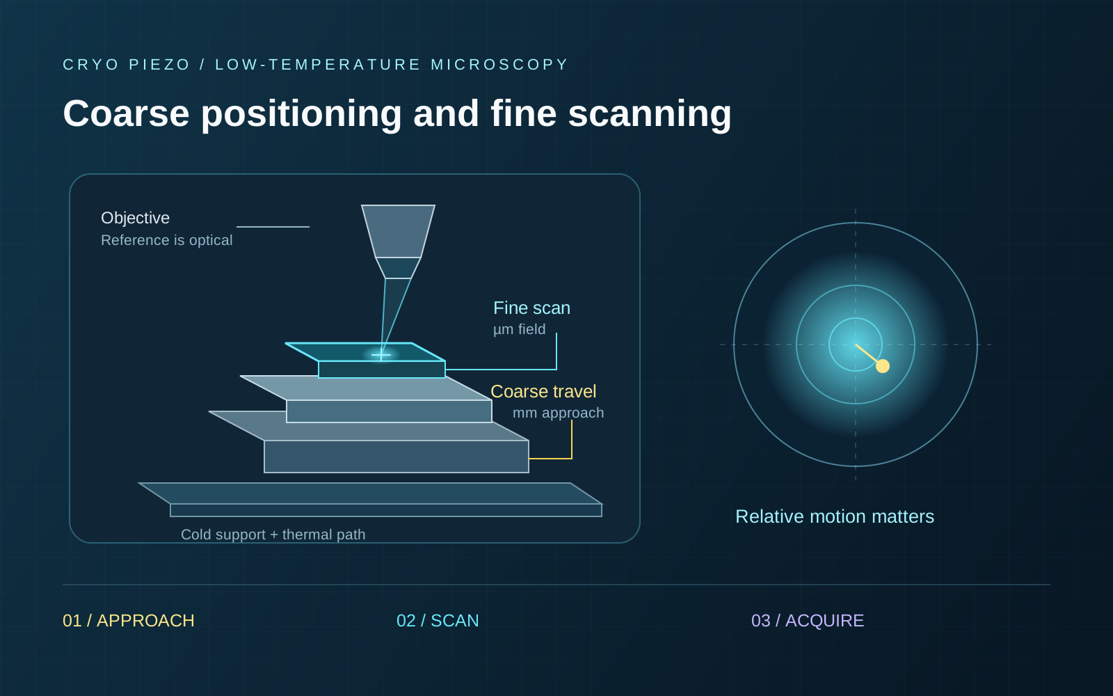
Use coarse travel to find a region, then a local scanner for imaging and alignment. Leave fine travel available for drift correction.
A published confocal microscope combines a piezotube scanner with three-axis coarse positioning. It is a useful architecture example. [1]
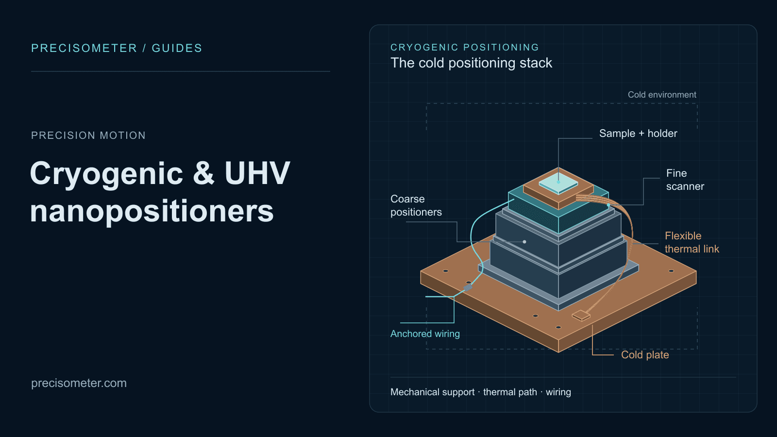
Our cryogenic range includes both motion scales. See environment selection and cryostat integration for mounting, thermal links and wiring.
Coarse positioning and fine scanning
| Task | What you specify | Relevant hardware |
|---|---|---|
| Find the region | Coarse XYZ reach, loaded motion and room for approach. | Linear positioners and the coarse controller. |
| Scan the target | Fine travel at temperature, calibration, sampling and timing. | Open-loop or capacitive-feedback flexure scanner. |
| Hold for acquisition | Relative motion over the measurement time and bandwidth. | The loaded stack, optical support, sensor and feedback configuration. |
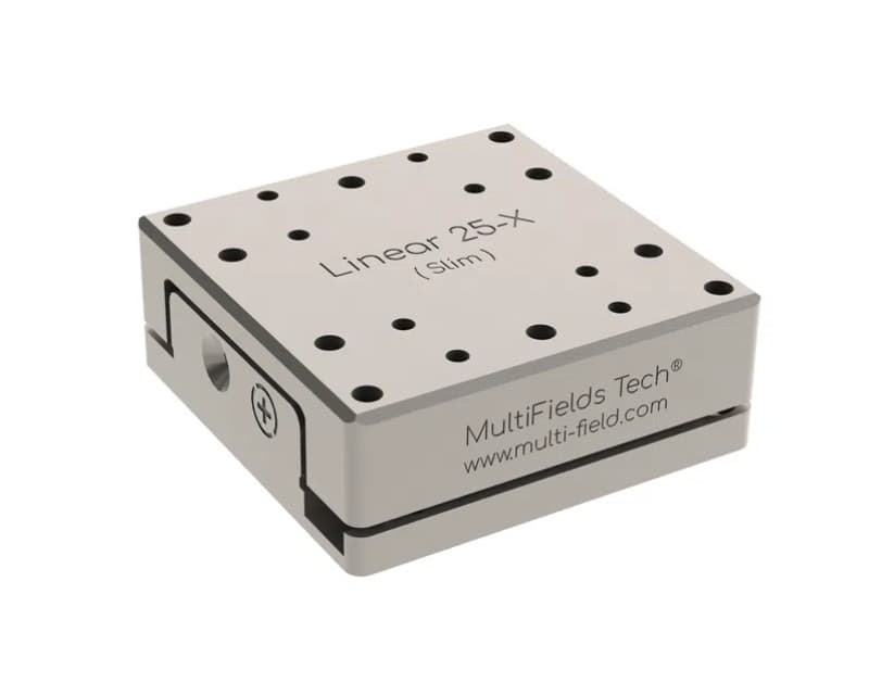
Linear25-x lists 6 mm travel, approximately 150 nm sensor resolution and 1–2 µm repeatability. Use the optical image and fine scan to locate the target after returning to its region.
Centre the local field within the scanner range. If correction travel runs out, reposition coarsely and register the image again.
How much travel is available cold?
Use the scanner’s travel at the operating temperature and drive voltage. A general ceramic contraction factor cannot establish the range of a complete stage. [3]
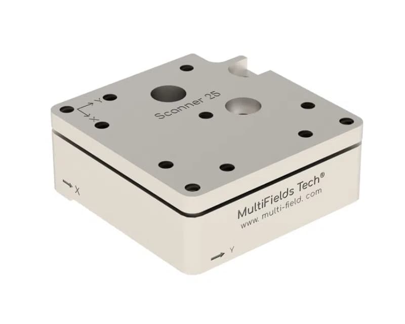
Scanner25-xy
55 × 55 µm at 300 K. Ask us for the range at your operating temperature.
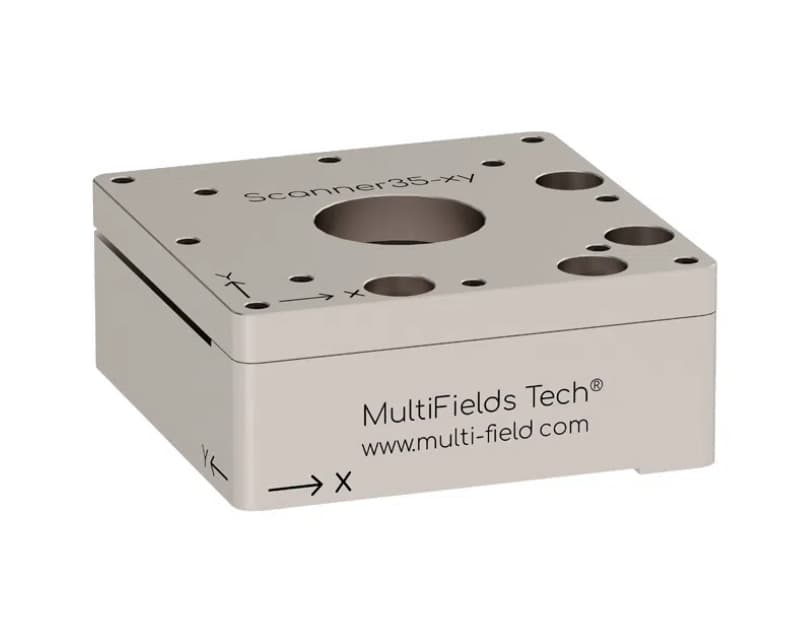
Scanner35-xy.Ultra
100 × 100 µm at 300 K; 60 × 60 µm at 4 K, with capacitive sensing. [5]
Allow margin for focus and drift correction. Below 4 K, confirm travel at the actual operating point.
Specify temperature, vacuum grade and magnetic field. Include holders, upper stages, adapters and cable forces in the load.
What does the feedback measure?
The stage sensor measures against its mechanical reference. Motion of an objective support or thermal joint outside that loop can still move the sample relative to the focus.
Liu and colleagues place the objective inside their cryostat to share sample/objective vibration. The design illustrates why relative optical motion matters. [2]
Open-loop local scanning
Suitable for a calibrated local scan with optical re-registration. Check reversal, creep and repeatability under the acquisition sequence.
Capacitive closed-loop scanning
Adds a stage displacement reference. Tune with the real load and include sensor noise and loop dynamics in the budget. [4]
Measure sample-to-focus motion over the acquisition time and bandwidth. Keep RMS jitter separate from peak-to-peak motion and slow drift.
Interactive / Optical alignment budget
Estimate drift and signal loss
Estimate signal loss for a Gaussian point target. Use measured motion where available; the presets are assumptions, not stage specifications.
End-of-hold relative signal
87.9%
Normalized to an aligned, jitter-free target. This is the local jitter average at the final drift offset, not the signal averaged over the full acquisition.
- Final relative offset
- 100.0 nm
- Initial signal with jitter
- 98.0%
- Offset at signal threshold
- 136.8 nm
- Modelled time to threshold
- 27.4 min
The model meets your threshold for this hold. Check measured target motion before choosing a recheck interval.
Calculation and assumptions
Model: I(r)/I₀ = exp(−ar²), a = 4 ln(2)/FWHM². Independent Gaussian X/Y jitter with standard deviation σ gives a normalized response exp[−ad²/(1+2aσ²)]/(1+2aσ²). Drift offset d = drift magnitude × duration. Assumes an initially centred, unsaturated point target, a stationary Gaussian jitter distribution and a fixed optical response. It omits axial motion, emitter brightness changes, temperature effects and feedback dynamics. Stage resolution and encoder noise are not substituted for measured relative motion.
A practical measurement sequence
- 01
Find after cooldown.
Find the region optically after cooldown; recheck focus and orientation.
- 02
Let the loaded system settle.
Track temperature and optical position after coarse motion. Measure the required settling delay.
- 03
Scan and centre locally.
Scan within the confirmed cold stroke, centre the target and leave correction margin.
- 04
Acquire.
Finish coarse stepping, then acquire with the drive and sensor state characterised for the experiment.
- 05
Recheck the reference.
Recheck an optical reference at a cadence set by measured drift. Separate movement from brightness changes.
Troubleshooting motion
| Observed behaviour | Useful comparison | What it helps distinguish |
|---|---|---|
| A target slowly leaves the field | Optical position versus time, temperature and recent motion history. | Slow relative drift, thermal recovery and scan-range exhaustion. |
| Forward and reverse maps differ | Repeat the same region with reversed scan direction and matched timing. | Calibration, hysteresis, creep, dynamics or a changing sample. |
| The encoder is quiet but the image moves | Measure a reference fixed to the sample in the optical image. | Motion outside the stage sensor loop. |
| A repeatable periodic pattern appears | Compare optical motion spectra with the cryocooler and drive timing. | Periodic coupling paths; frequency alone does not prove their origin. |
Compare cryogenic stages
Start with coarse travel, local scan field and feedback. We can check adapters, axis order and optical clearance for your cryostat.
Coarse positioning
Linear25-x
6 mm coarse X travel for reaching regions after cooldown. Locate the target with the optical signal and fine scanner.
- Travel range
- 6 mm
- Max. Load
- 500 g
- Sensor resolution
- ~150 nm
- Published repeatability
- 1-2 um
Open-loop XY scanning
Scanner25-xy
Compact open-loop XY scanning. The 55 × 55 µm range is at 300 K; confirm the field at your temperature.
- Travel range @300 K
- 55 x 55 um
- Max. Load
- 200 g
- Drive Voltage
- Max. 75 V @300 K, Max. 180 V @4 K
XY scanning with feedback
Scanner35-xy.Ultra
Capacitive-feedback XY scanning with 60 × 60 µm travel at 4 K. Pair with the Ultra controller and required environment grade.
- Travel range
- @300 K: 100 x 100 um; @4 K: 60 x 60 um
- Max. Load
- 500 g
- Sensor
- Capacitive displacement sensor
- Resolution
- 0.5 nm
Confirm cold travel, repeatability conditions and the exact temperature/vacuum suffix in the quotation.
Include the matching drive and sensor chain
- MC-NewtonLT.06 — the coarse multi-axis controller option for the cryogenic positioner chain.
- MC-ArchimedesLT.03 — the controller family for the open-loop cryogenic scanners.
- MC-ArchimedesLT.03.Ultra — the capacitive-feedback controller for the Ultra scanner chain.
- FTC25.L** or FTC35.L**, with the appropriate mounting adapters — specify the thermal and mechanical connections for the selected stage family.
Before stacking stages, check interfaces and the load on each lower axis, including everything mounted above it.
From optical target to cold positioning
Choose stages for your cryostat
Send the cryostat envelope, temperature, cold scan field, payload and acquisition time. Include optical geometry and any measured drift or vibration.
Request a cryogenic positioning configurationQuestions before choosing a stage
Can I use room-temperature travel for a 4 K map?
Use the cold specification. Scanner35-xy.Ultra lists 100 × 100 µm at 300 K and 60 × 60 µm at 4 K. Confirm travel again below 4 K.
Does 0.5 nm resolution guarantee a stable optical target?
No. Measure relative sample-to-focus motion over the acquisition time and bandwidth, including motion outside the sensor loop.
Do all cryogenic stages work at 30 mK and in UHV?
Choose the exact grade: standard cryogenic, ULT, UHV or combined UHV.ULT. Confirm the complete sensor and wiring configuration.
Should I choose open-loop or closed-loop scanning?
Open loop can suit calibrated local scans. Capacitive feedback adds a position reference. Compare cold travel, noise, bandwidth and return requirements.
References and datasheets
- [1]Development of a confocal scanning microscope for fluorescence imaging and spectroscopy at variable temperatures
Hu, Moran and Woehl (2019), Review of Scientific Instruments 90, 043702. A published microscope architecture combining coarse low-temperature positioning with a local piezo scanner.
- [2]Cryogenic photoluminescence imaging system for nanoscale positioning of single quantum emitters
Liu et al. (2017), Review of Scientific Instruments 88, 023116. Objective/sample geometry and common-mode vibration in cryogenic optical measurements.
- [3]Temperature-dependent behavior of piezo actuators
PI Ceramic, technology reference. Temperature-dependent displacement; it does not establish a universal cold-range multiplier for a finished stage.
- [4]Piezo controllers and piezo drivers
Physik Instrumente, technology reference. Position feedback, controller tuning and dependence on the payload and mechanical system.
- [5]Cryogenic Motion — Scanner.Ultra
MultiFields, manufacturer product information; see linked Precisometer model sheets for the quoted configuration. Scanner architecture, capacitive sensing, temperature-dependent travel and environment variants.
Product cards link the model sheets. Research examples and the optical model illustrate design choices; their performance is not a stage specification.