Planar PIV · 2D2C
One camera, one light sheet
Measure two in-plane velocity components. A practical starting architecture for an accessible seeded flow. Motion normal to the sheet can remove particle pairs.
Flow measurement · Application guide
Turn a field of view and flow speed into laser timing, camera requirements and light-sheet optics. Build a practical PIV shortlist with Precisometer.
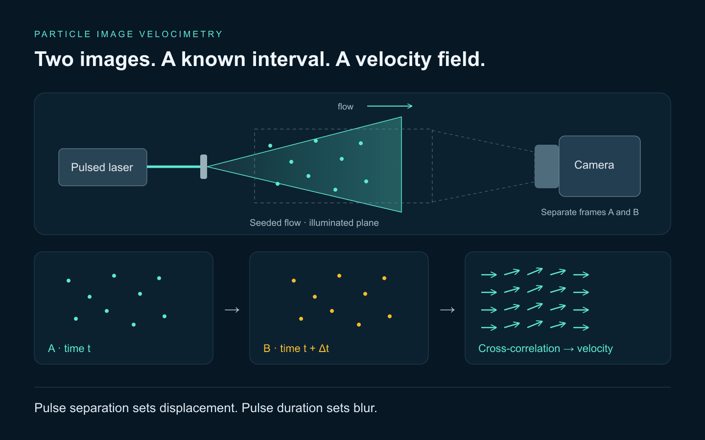
01 / From particles to velocity
A light sheet illuminates tracers carried by a liquid or gas. Record their scattered light twice, with a known interval Δt. Cross-correlate small interrogation windows in the two images to estimate local displacement; calibration turns pixels into distance, and distance divided by Δt gives velocity.
s = field width / sensor pixels
U = displacement × s / Δt
b = U × pulse duration / s
PIV follows a group pattern. Particle tracking velocimetry (PTV) instead follows individual particles. In either case, the tracer must follow the fluid closely enough for the experiment: particle inertia, buoyancy and settling can introduce differences between particle and fluid velocity.
One camera, one light sheet
Measure two in-plane velocity components. A practical starting architecture for an accessible seeded flow. Motion normal to the sheet can remove particle pairs.
Two calibrated camera views
Recover three velocity components within the illuminated plane. Add angular-view calibration, suitable focus geometry and matched acquisition timing.
Multiple views of a volume
Reconstruct a three-dimensional region using an appropriate multi-camera method. It requires different illumination, calibration and processing from a planar setup.
Measurement background: Dantec’s PIV measurement principles and LaVision’s planar and volumetric PIV overview (PDF).
02 / Interactive timing lab
Pulse separation decides how far a pattern moves between images. Pulse duration decides how far it smears within each image. Changing one does not fix the other. Explore both at your actual image scale.
Use a representative fastest region. Inputs explore geometry; they do not describe a guaranteed laser or camera operating mode. For CW illumination, τ is the effective camera exposure.
One particle pattern, two times
32 × 32 sensor-pixel view
Solid trails show motion during each exposure; dashed lines join exposure centres. Trails are clipped at the view edges. Particle thickness and brightness are schematic.
Single particle · 8× close-up
Blur: 0.041 px
Dashed circle: no motion. Amber line: travel during τ. At the default settings, the blur is only 0.041 px; increase τ to see the trail grow.
Displacement is within the illustrative 2–8 px starting range. Verify particle count, gradients, out-of-plane loss and correlation quality on actual images.
Motion blur is within this lab’s 0.5 px design target. A pulse or effective exposure of 2441.41 ns gives 0.5 px blur at this scale. The target is an engineering choice, not a universal PIV limit.
s = W/N; Δx = UΔt/s; b = Uτ/s
Use consistent length and time units. W is horizontal object-space field width, N is sensor width, U is in-plane speed. Constant speed and uniform image scale are assumed.
L = ns; g = 0.5ns; Δt₆ = 6s/U
n is the final window width in pixels; L is its footprint and g is vector spacing at 50% overlap. Grid spacing is not independent spatial resolution. No photon budget, tracer response or uncertainty is predicted.
Try roughly 2–8 pixels between frames, then assess real correlation quality. The classical quarter-window rule is a starting point for single-pass processing; multi-pass window deformation changes that constraint. The calculator’s 0.5-pixel blur target is a conservative design choice.
At 50% window overlap, adjacent vectors are spaced by half a window. Their sampled regions overlap, so those vectors are correlated. The window footprint, tracer images, sheet thickness and velocity gradients all affect the detail you can resolve.
Processing reference: PIVlab’s interrogation-window and displacement guidance.
Worked example / 100 mm field · 2048 pixels · 10 m/s
Sampling is 48.8 µm/pixel. A 200 ns pulse produces about 0.041 pixel of blur; a 32-pixel final window covers 1.56 mm and gives 0.78 mm vector spacing at 50% overlap. That is a useful starting geometry for evaluating the DPS-527-PIV, provided its paired-pulse energy and your camera timing are suitable.
Change to a 10 mm field at 100 m/s and the same 200 ns pulse gives 4.10 pixels of blur. A 6-pixel displacement then needs about 0.293 µs separation and the 0.5-pixel blur target requires about 24 ns illumination or shorter. This case calls for a shorter-pulse source and a camera proven at that image interval.
03 / Specify the measurement chain
For slow flows, CW illumination can work if the camera exposure is short enough and the available light gives usable particle images. For faster motion, short pulses provide the effective exposure. Compare energy per pulse at the chosen repetition rate, pulse duration, beam profile, pointing, trigger behaviour and energy balance between pulses.
Green sources around 527–532 nm are practical candidates for visible scattering and silicon cameras. Wavelength still depends on tracer response, absorption, filters and optical access. Average watts alone cannot establish useful energy in each image.
Prefer monochrome raw capture when it suits the signal. Specify the full field, pixel count, sensitivity at the laser wavelength, lens coverage and aperture. A global shutter simplifies full-frame timing; a rolling shutter needs a documented common exposure interval for pulsed illumination.
A 100 fps headline means 10 ms between conventional consecutive frames. It does not establish whether the camera can record two images 30 µs apart. Ask for minimum interframe time, dead time and a supported double-frame or frame-straddling mode. Confirm performance at your ROI, bit depth and interface.
A cylindrical lens or appropriate sheet-forming assembly spreads light across a plane. Specify sheet height, thickness through the measurement region, working distance and usable uniformity. Beam quality and divergence affect how thickness changes along propagation; the thinnest waist is not the whole illuminated field.
A very thin sheet rejects background but loses particles sooner when they move out of plane. Compare out-of-plane travel |w|Δt with sheet thickness. Account for window refraction, wall reflections and actual collected signal when choosing optics and filtering.
Use one timing reference for camera exposures and laser firing. Verify trigger polarity, levels, latency, jitter and the optical delay between pulses. Record one intended illumination event in each frame and confirm the sequence with exposure outputs and an optical timing measurement.
The interval within a pair and the velocity-map acquisition rate are separate requirements. A 30 µs pair captured 10 times per second does not resolve a continuous high-frequency flow history. Time-resolved measurements also need adequate sustained camera, laser, storage and processing rates.
04 / Precisometer devices & components
Start with the illumination source, then match sheet delivery, imaging and mechanical support to the same experiment.
Pulsed green illumination
A dedicated PIV laser candidate for experiments needing green pulses and configurable paired illumination.
527 nm
Green output
~200 ns
Pulse duration at 1 kHz
Request energy in each pulse, achievable minimum separation, energy balance and timing jitter at your selected rate. The single-pulse energy specification does not promise two 20 mJ pulses at every delay or the full energy range at 10 kHz.
Illuminate the test section
Explore CW and pulsed sheet-source configurations. Specify the wavelength, field height, sheet thickness and working distance so we can propose the optical delivery.
Explore sheet-source optionsRecord the particle pairs
Use our camera catalogue to define sensor format, sensitivity and acquisition rate. For PIV, ask us to verify the exact trigger mode and minimum image interval before selecting a model.
Compare camera optionsKeep the geometry stable
Build stable support for sheet optics, steering mirrors and the camera. Match beam height, clear aperture and mechanical access; check optical coatings and pulse-energy limits separately.
Explore mechanical componentsConsidering the DPS-1064-PIV? Its 1064 nm output needs a detector, filters and sheet optics chosen for that wavelength; it is not a direct optical replacement for a green source. Ask us to confirm the current configuration and specifications.
Specification source: DPS-527-PIV manufacturer datasheet. Product suitability and the proposed system scope require application-specific confirmation.
05 / From first images to useful data
Image a target of known dimensions at the light-sheet location through the same windows and lens configuration. Correct relevant distortion. Stereo and volumetric methods need their own multi-view calibration.
Inspect particle-image size, density, brightness and saturation across the field. Balance scattering strength against flow-following response. Keep tracer properties and any fluorescence filters in the experiment record.
Verify actual optical separation and that each intended pulse lands in its own recorded exposure. Save raw image pairs with acquisition settings and pair-rate information. Test sustained capture for dropped or mispaired frames.
Mask solid boundaries, use a suitable coarse-to-fine processing sequence, and inspect correlation and rejected-vector patterns. Retain validation settings; compare with a known motion or independent reference where possible.
| What you see | Likely mechanism | What to check |
|---|---|---|
| Long streaks in raw frames | Particles move during illumination. | Shorten the laser pulse or effective camera exposure; check blur in pixels before increasing power. |
| Weak or missing correlation | Too few paired particles, excessive displacement or particles leaving the sheet. | Inspect raw image pairs. Adjust seeding, separation, sheet thickness or initial window size; verify both pulses were recorded. |
| Bright stationary patches | Wall reflections or background dominate. | Rework optical access, masking and wavelength filtering. Avoid saturation and preserve the original raw images. |
| Row-dependent illumination | The pulse missed the common exposure interval. | Verify shutter mode and exposure timing across the full sensor. Check both frames at the intended ROI and bit depth. |
| A dense map with little real detail | Small vector spacing is being mistaken for resolution. | Check final interrogation footprint, particle count and gradients. Greater overlap creates more correlated samples. |
Talk to Precisometer
Share your measurement geometry and required timing. We can help shortlist a laser, sheet optics, imaging and mechanical components, and clarify the equipment and integration included in the proposal.
Include with your enquiry
Practical answers
PIV estimates velocity from the displacement of tracer-particle image patterns between two known times. Planar PIV uses a light sheet and one camera to measure two in-plane velocity components; stereo PIV uses two calibrated views to recover three components in that plane.
Slow flows can be measured with continuous illumination if a short camera exposure freezes the particles and the camera provides a suitable image interval. Faster flows usually need short laser pulses and synchronized acquisition. Pulse separation sets displacement; pulse duration sets motion blur.
No. Frame rate alone does not establish the minimum separation between two separately recorded exposures. Confirm shutter behaviour, interframe dead time, trigger latency and jitter, exposure outputs, raw image access and software support for the exact camera mode.
It is a candidate for green pulsed illumination: its datasheet specifies 527 nm, 1–20 mJ single-pulse energy at 1 kHz, approximately 200 ns pulses at 1 kHz, and a nominal 0–500 µs double-pulse delay. Check motion blur at your velocity and image scale, and request energy, timing and repetition-rate specifications for the exact paired-pulse operating point.
This guide links to laser sources, light-sheet assemblies, camera selection and optomechanics offered through Precisometer. Ask us to define the proposed supply scope, including camera compatibility, synchronizer, seeding, calibration target, acquisition software, processing software and commissioning.
Before you specify
Explore camera selection, laser specifications and the mechanical stability behind repeatable optical measurements.
 Scientific cameras
Which sensor technology your photon flux actually needs, why rolling and global shutter answer different questions, and how to check the data can leave the camera at all.
Open guide Photonics
Linewidth, spectral width, RIN, M², and coherence length answer five different questions. Translate each into the units your experiment is designed in — and learn which ones not to pay for.
Open guide Opto-mechanics
Vibration, thermal drift and mechanical integration are one problem. Budget the motion at the sample, then specify the table, the isolation, the mounts and the beam height that budget asks for.
Open guide