✕
17.3 µmOpen-loop, voltage drive
open loop- Hysteresis
- 15.0 µm
- Creep
- 2.25 µm
- Sensor noise
- 0.30 nm
Nanopositioning · 18 min
An open-loop piezo is not a worse closed-loop piezo. It is a different instrument — faster and quieter, and wrong by 15 % of its travel. Knowing which of those facts matters to you is the whole decision.
Start here
A piezoelectric actuator converts field into strain with sub-nanometre smoothness and essentially infinite resolution. That part is genuinely remarkable, and it is why piezos own the nanometre regime. What they do not do is tell you where they are.
The relationship between applied voltage and displacement is neither single-valued nor stable. It is single-valued only if you ignore history — the extend and retract paths differ by 10 to 15 percent of full travel. It is stable only if you ignore time — displacement continues creeping logarithmically for minutes after the voltage settles. Neither of these is a defect in a particular stage; both are ferroelectric physics, and every PZT actuator has them.
Closing a loop around a position sensor removes both. The mistake is concluding that closed loop is therefore better. A servo buys accuracy with two currencies: it writes its sensor noise onto your position, and it forces the usable bandwidth well inside the mechanical resonance. For a great many applications — anything scanning a repeatable trajectory at speed — that is a bad trade, and the open-loop stage with a linearisation model is the better instrument.
The four error terms
| Mechanism | Typical scale | Behaviour | Fixed by | What it is |
|---|---|---|---|---|
| Hysteresis | 10–15 % of full-scale travel | Path-dependent, rate-independent | Servo, charge drive, or an inverse model | The extend and retract branches of the voltage–displacement curve do not coincide. Where you are depends on where you came from, so the same command voltage gives two different positions. |
| Creep | 1–2 % of the step, per decade of time | Logarithmic in time after a move | Servo only | Displacement keeps growing after the voltage has settled. Invisible in a fast scan, ruinous in a long exposure — and the one term feedforward linearisation does not touch. |
| Nonlinearity | 1–2 % of full scale | Deterministic, repeatable | Servo or calibration | Even ignoring the hysteresis loop, strain is not proportional to field. Because it is repeatable, a lookup table handles most of it without any sensor. |
| Thermal drift | Structure-dependent, often tens of nm/K | Slow, follows the room | Neither, unless the sensor spans the same loop | The term that beats all of the above in practice. A servo only corrects drift inside its metrology loop — everything between the sensor and your sample is uncontrolled. |
The highlighted row is the one that beats all the others in most real instruments, and it is the one a servo does least about — feedback only corrects drift inside its own metrology loop.
Interactive
Set your travel, your move size, how long you hold, and what accuracy you actually need. The panel evaluates every drive strategy against that target at once. Two things usually surprise people: how badly hold time punishes open loop, and how much residual error a closed-loop stage still carries when the actuator is oversized.
All five options priced in the same currency: total positioning error against your target. Watch what happens to the open-loop rows when you extend the hold time.
100 µm
Hysteresis scales with this, not with the move you command — so oversizing the actuator costs accuracy.
50 % of range
Creep scales with the size of the step you just took.
1.7 min
Creep grows with the logarithm of time. A fast scan never sees it; a long exposure does.
10.0 nm
What your application actually needs, not what the datasheet advertises.
Cheapest option that meets target
None of them
Loosen the target, shorten the hold, or choose a shorter-travel actuator — full-scale range is driving the error.
Reading this budget
Nothing on this list reaches 10.0 nm at 100 µm of travel. Look at the linearity column: even capacitive feedback leaves a residual that is a fixed fraction of full scale. The fix is a shorter-travel actuator, not a better sensor — halving the range halves that error term.
Representative coefficients for PZT flexure stages: hysteresis 10–15 % of full scale open-loop, creep 1–2 % per decade of time, closed-loop linearity 0.1–0.2 % with strain gauges and 0.02–0.05 % with capacitive sensors. Real figures vary by stage, drive amplitude, preload and temperature — take them from the datasheet of the actual model. Hysteresis and creep are summed linearly and noise added in quadrature, so totals are worst-case. Thermal drift of the surrounding structure is not included and frequently exceeds everything shown here.
If you close the loop
Every closed-loop stage runs essentially the same control law. What separates a good one from an adequate one is what it is measuring, and how directly.
The sensible default. Compact, inexpensive, no extra volume in the stage. It measures flexure strain rather than your position, so it infers rather than observes.
Buy this when the position is the measurement. An order of magnitude better linearity, far quieter, and it observes the moving platform directly. Costs real money and volume.
The route to long travel. This is what the stick-slip motor stages use to hold nanometre resolution over tens of millimetres, where a flexure sensor has no reach.
A closed loop holds the sensor reading constant. Everything between that sensor and the thing you actually care about — the sample, the fibre, the focal plane — sits outside the loop and drifts freely.
In a typical microscope or alignment station that uncontrolled path is longer than the controlled one. If your position drifts overnight with a closed-loop stage installed, suspect the mounting, the mounts and the table before you suspect the stage. The rig guide covers that budget.
Piezo coefficients fall substantially on cooling. A flexure scanner giving 40 × 40 µm at room temperature gives roughly 24 × 24 µm at 4 K — so specify the range at your operating temperature, not at 300 K, or you will arrive at base temperature with a stage that no longer reaches.
Sensor choice shifts too. Strain-gauge factors are temperature dependent and drift as the system cools, while capacitive sensing degrades much more gracefully. Cold is one of the clearer cases for paying for capacitive feedback. More on cryogenic and UHV selection.
Interactive
Accuracy is only half the trade. Add your payload — which pulls the resonance down as the square root of mass — and your target scan rate, then check whether the amplifier can actually supply the current. That last term stops more fast scans than the mechanism does, and it appears on no stage datasheet.
Closing the loop buys accuracy and spends bandwidth. Add your payload and your target scan rate, and see which strategies are still on the table — then check whether the amplifier can supply the current either of them needs.
1.00 kHz
From the datasheet, always quoted unloaded. Flexure scanners run 100 Hz to a few kHz.
50 g
The mass the piezo already carries before you add anything.
150 g
Objective, sample holder, mirror, fibre chuck — whatever you bolt on top.
100 Hz
Frame rate for a raster, step rate for a z-stack, loop rate for stabilisation.
3.0 µF
Large-travel actuators are large capacitors. This is what the amplifier has to drive.
150 V pp
Full-scale swing. Scanning a fraction of the range proportionally cuts the current.
Loaded resonance
500 Hz
50 % below unloaded
Open-loop usable
167 Hz
≈ resonance / 3
Closed-loop bandwidth
100 Hz
≈ resonance / 5
At 100 Hz
Both strategies work
Your target sits inside the servo bandwidth, so you can close the loop and keep the speed. Choose on accuracy and noise instead, using the budget panel above.
Amplifier current required
I_peak = π · f · C · V_pp
At your target, 100 Hz
141 mA
peak, full-scale sinusoid
At the open-loop ceiling
236 mA
what a full-speed scan demands
Within the reach of an ordinary piezo amplifier. Note that this scales linearly with frequency, capacitance and swing together — a large-travel actuator is a large capacitor, so pushing travel and speed at once escalates the amplifier quickly.
The payload term people forget
Adding 150 g to a 50 g stage drops the resonance by 50 %, from 1.00 kHz to 500 Hz. Resonance goes as the square root of mass, so it is unforgiving in both directions — a heavy objective or a chunky fibre chuck can halve your usable bandwidth before any control decision is made. Specify the stage against the loaded resonance, never the datasheet number.
First-order lumped model: single dominant mode, rigid payload, no notch filtering. Real controllers with input shaping or notch filters exceed the resonance/5 rule, and a poorly mounted payload with its own compliance can do considerably worse. Current is the peak for a full-scale sinusoid; triangular scans demand more at the turning points.
The short answer
You repeat the same path thousands of times, so an inverse model or a calibrated lookup table removes the hysteresis once. Keeping open-loop bandwidth and noise is worth more than absolute accuracy you never use.
There is no trajectory to calibrate against. You commanded 12.400 µm and you need to be at 12.400 µm regardless of history — that is precisely what hysteresis prevents open-loop.
Creep grows with the logarithm of hold time and is the one error a feedforward model cannot anticipate. Anything holding for minutes needs a servo, or needs to re-reference.
Servo stability forces the loop well inside the mechanical resonance. Driven open-loop you can run a smooth trajectory considerably faster before ringing takes over.
Counterintuitive but real: a servo writes its sensor noise onto the position. An open-loop actuator driven by a quiet amplifier can be the more stable of the two on short timescales.
You need the position to be observed rather than inferred, with linearity good enough that the stage is not the dominant uncertainty in your result.
From the catalogue
Every figure below is from the model’s own specification. Where a range or resonance is quoted under a stated condition — loaded, or at temperature — that condition is given, because those are the numbers that describe your instrument rather than the datasheet.
The cryogenic scanner line splits exactly along this guide: an open-loop flexure scanner, and an Ultra variant with capacitive feedback. Note the travel figures — piezo coefficients fall substantially on cooling, so a scanner that gives 40 µm at room temperature gives 24 µm at 4 K. Budget the range at your operating temperature, not at 300 K.
The controller that makes the choice reversible: it accepts either sensor type for closed-loop operation and will equally drive a scanner open-loop. If you are not yet sure which side of the trade your application sits on, this is the hardware that lets you measure it rather than guess.
Capacitive feedback into a 50 kSa/s realtime loop. The sample rate matters more than it looks: loop rate sets how much of the mechanical bandwidth the servo can actually use, and a slow loop turns a fast stage into a slow one. Capacitive sensing is also the right choice cryogenically, where strain-gauge factors drift with temperature.
A worked example of everything in the dynamics panel. The 250 Hz figure is quoted at 150 g of objective, not unloaded — which is the honest way to specify it, and rarer than it should be. A 250 Hz loaded resonance gives roughly 50 Hz of closed-loop bandwidth, so z-stack step rates above that are not available regardless of the controller.
The standard scanner modules, where the trailing .C denotes the closed-loop build. Choose the shortest range that covers your travel — residual linearity error is a fixed percentage of full scale, so a 100 µm scanner used over 80 µm is materially more accurate than a 300 µm scanner doing the same job.
A 2 kHz resonance is the fastest thing in the piezo catalogue, and beam-steering loops are exactly where the bandwidth cost of a servo has to be argued rather than assumed. Worth reading alongside the dynamics panel: at this resonance a closed loop still leaves several hundred hertz, which is enough for most stabilisation work.
Where flexure scanners run out of range, stick-slip piezo motors with optical encoders take over — millimetres of travel at nanometre resolution. Different mechanism, same lesson: the encoder is what makes the number real, and the open-loop stick-slip step size on its own is neither repeatable nor linear.
If you are not certain which side of the trade you are on, the productive move is to specify a controller that supports both and measure it on your own trajectory. Tell us the travel, the payload, the scan rate and the accuracy you need and we will size the stack.
The rest of the stack
The half of the decision that lives outside the stage. Sensor type, loop rate and available current decide how much of the mechanism you can actually use.
Scanner modules, objective scanners, parallel platforms and the MC-Newton and MC-Archimedes controllers that drive them.
Configure axes, travel and feedback against each other rather than picking a model number and hoping.
Open-loop scanners and closed-loop Ultra variants, with the thermal links and adapter plates that a cold stack needs.
Controllers, drivers and interfaces across the motion range, including multi-axis synchronisation.
For closing a loop against your own detector — the case where the position error comes from your experiment rather than from a stage sensor.
One specification to insist on that rarely appears: the controller loop rate. A capacitive sensor with a 1 kHz loop cannot service a 2 kHz mechanism, and you will have bought bandwidth you cannot reach. Ask for the realtime loop rate and the sensor bandwidth separately.
A piezo covers micrometres. Almost every real instrument needs coarse travel underneath it, and the interface between the two is where accuracy is usually lost.
Millimetre-to-centimetre travel underneath the piezo. Coarse capture range so the fine axis only ever works over its linear span.
Set-and-forget adjustment for axes that are aligned once at build time and never scanned.
Motorized linear, vertical, rotation, and multi-axis positioning systems.
The classic coarse-plus-fine application: manual stages for capture range, closed-loop piezo for the last micrometre.
A servo only corrects what its sensor spans. Everything outside that loop — including the table — is uncontrolled drift.
Common questions
No, and treating it as strictly better is the most common specification error in this area. A servo removes hysteresis and creep, and in exchange it writes sensor noise onto your position and forces the usable bandwidth well inside the mechanical resonance — typically to about a fifth of it, against roughly a third for a smooth open-loop trajectory. If you scan a repeatable path at speed, or you need the quietest possible position on short timescales, open-loop with an inverse-hysteresis model can be the better instrument. If you must reach an absolute coordinate, or hold position for minutes, you need the servo.
Typically 10 to 15 percent of full-scale travel for a PZT actuator driven by voltage. The critical detail is that it scales with the full range of the actuator, not with the move you commanded — so a 2 µm step inside a 100 µm actuator can carry 10 to 15 µm of positional ambiguity depending on the history of the drive. It is also path-dependent rather than a fixed offset, which is why it cannot be calibrated out with a single number, only with a model of the loop.
After a voltage step the displacement keeps growing, logarithmically in time, as domains in the ceramic continue to reorient. A common model is that displacement grows by 1 to 2 percent of the step per decade of time, referenced to about 0.1 s. That means roughly 3 to 6 percent of the step after 100 seconds, and more after an hour. It is invisible in a fast raster and dominant in a long exposure, and it is the one error term that feedforward linearisation does not fix — a model can anticipate hysteresis because it depends on the path, but creep depends on how long you have been waiting.
Strain gauges are the sensible default: compact, inexpensive, no extra volume, and 0.1 to 0.2 percent of full-scale linearity is enough for most positioning. Capacitive sensors give roughly an order of magnitude better linearity at 0.02 to 0.05 percent, lower noise, and better thermal behaviour, because they measure the gap to the moving platform directly rather than inferring position from strain in a flexure. Buy capacitive when the position is itself the measurement, when you are working cryogenically where gauge factors drift, or when the stage would otherwise be the dominant uncertainty in your result.
Partly. Two approaches work. Charge drive — regulating charge into the actuator instead of voltage — reduces hysteresis by roughly an order of magnitude because strain tracks charge far more linearly than it tracks field; it complicates DC holding and is uncommon in commercial controllers. Inverse hysteresis modelling, using a Preisach or Prandtl–Ishlinskii model applied as feedforward, gets similar improvement in software and keeps full open-loop bandwidth and noise. Neither addresses creep, so both suit fast repeatable trajectories rather than long holds.
Resonant frequency goes as the square root of stiffness over mass, so adding load pulls it down as the square root of the total moving mass. Adding 150 g to a 50 g moving stage takes the resonance to half its unloaded value. Datasheets quote the unloaded figure almost universally, so the usable bandwidth of your actual assembly is typically well below the number you bought against. Specify against the loaded resonance, and be sceptical of any objective scanner or steering mirror whose resonance is not quoted with a stated load.
Three things in turn, and the last one surprises people. Mechanical resonance sets the ceiling — roughly resonance over three open-loop, over five closed-loop. Servo loop rate can bite before that if the controller cannot sample fast enough to use the mechanism. And then the amplifier: a piezo is a capacitor, so a full-scale sinusoid draws a peak current of pi times frequency times capacitance times voltage swing. A 3 µF actuator swung 150 V at 1 kHz needs about 1.4 A, which is beyond many benchtop amplifiers. That constraint appears on no stage datasheet because it belongs to the controller.
Only inside its own metrology loop. A servo holds the sensor reading constant, which means it corrects drift in everything between the sensor and the actuator — and corrects nothing between the sensor and your sample, your optic or your fibre. In many instruments that uncontrolled path is longer than the controlled one, and thermal drift there exceeds every error term in this guide. If your measurement drifts overnight with a closed-loop stage installed, the stage is probably not the problem.
Keep reading
Stage technology selection, cryogenic and UHV constraints, the drift budget around the stage, and one application where all of it comes together.
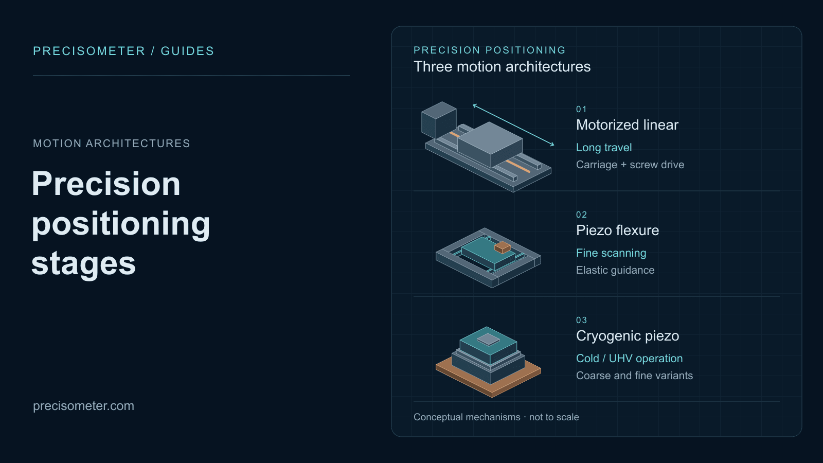 Precision motion
Match travel, resolution, speed, load, vacuum, temperature, and magnetic field requirements to motorized linear, ambient piezo, or cryogenic piezo positioning architectures.
Open guide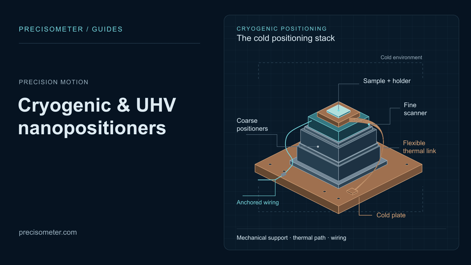 Precision motion
Translate temperature, pressure, travel, payload, feedback, and motion requirements into a defensible cryogenic-stage shortlist.
Open guide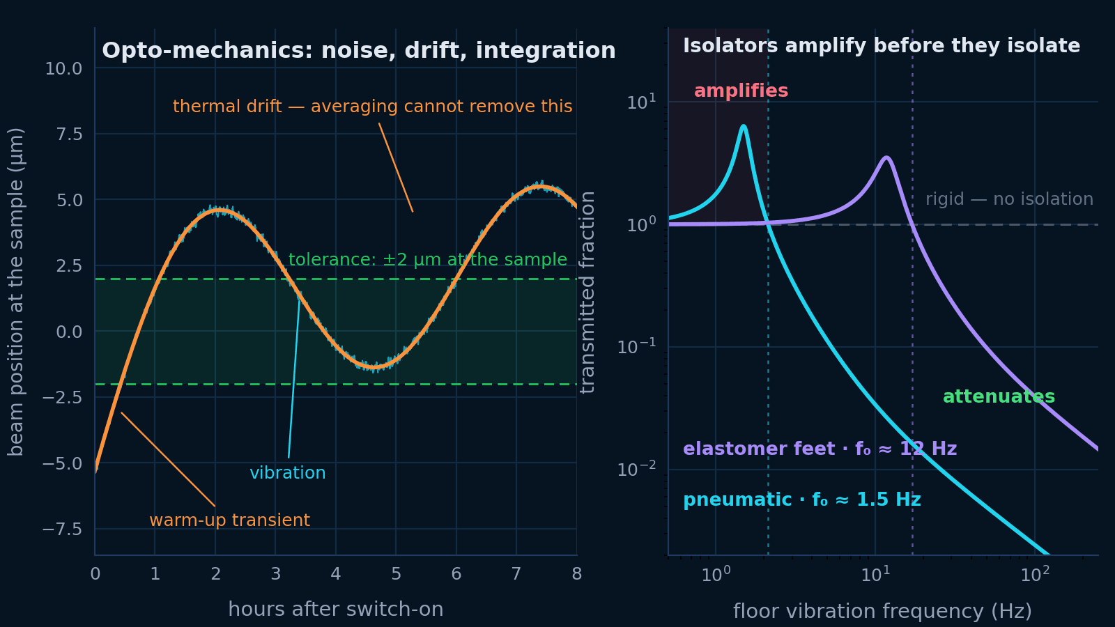 Opto-mechanics
Vibration, thermal drift and mechanical integration are one problem. Budget the motion at the sample, then specify the table, the isolation, the mounts and the beam height that budget asks for.
Open guide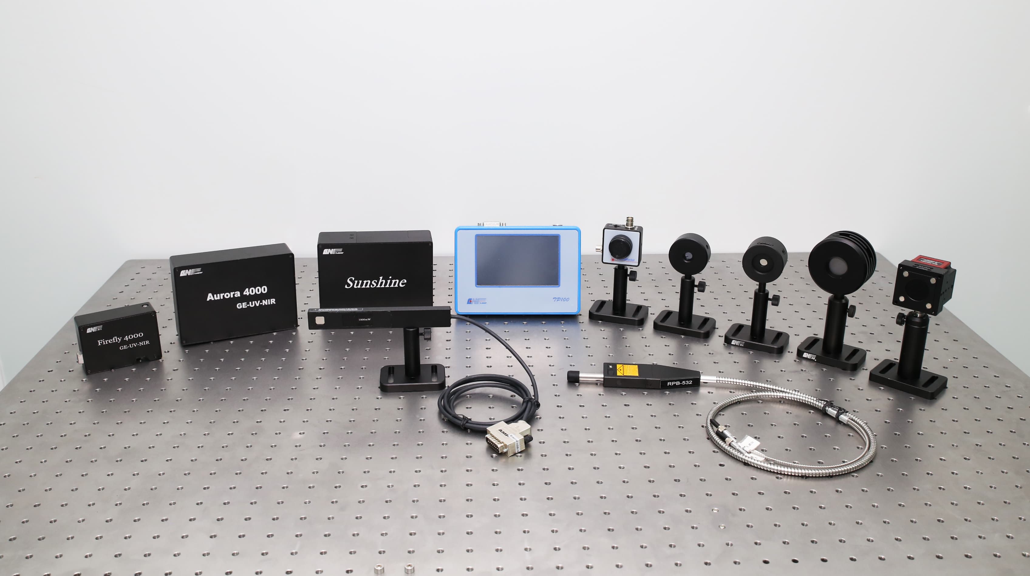 Integrated photonics
Turn fibre-to-chip coupling tolerance, polarization, device Q, and port count into a complete source, detection, coarse-alignment, and closed-loop nanopositioning stack.
Open guideRequired travel, positioning accuracy, hold time, payload mass, scan rate and environment — ambient, vacuum or cryogenic — are enough for us to work back to a stage, a feedback strategy, a sensor type and a controller that can actually service it.