01 · Two experimental questions
Two questions, one kind of record
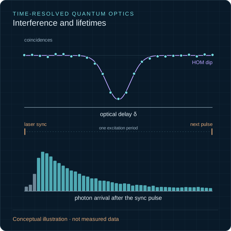
Will these two photons interfere?
Measure coincidences while adjusting their relative arrival time.
Go to the applicationHow quickly does this quantum emitter decay?
Measure photon arrival times relative to excitation pulses.
Go to the applicationBoth answers come from timing. A time tagger records the time and the input channel of every electrical pulse it receives, from a single-photon detector or from a reference signal such as a laser's synchronization output. Coincidences and decay curves are computed from those records.
02 · The timing chain
From detector pulse to histogram — and where the FPGA fits
Input electronics detect the edge of each pulse. A time-to-digital converter (TDC) measures when it happened against a shared reference clock.
A field-programmable gate array (FPGA) is configurable digital hardware that handles many operations in parallel. Depending on the design, it implements the timing measurement itself or works with a separate TDC. It formats timestamps, merges channels, buffers data, keeps inputs synchronized and, where the instrument supports it, runs real-time processing. Software then turns timestamps into coincidence measurements and arrival-time histograms.
Detector / laser sync
- Photon detector pulses
- Laser sync pulses, for pulsed excitation
Inside the time tagger
Input electronics
- Threshold and edge detection on each channel
Timing measurement
- TDC: time of each edge against a shared reference clock
Event processing
- FPGA: channel + timestamp
- Buffering, channel merging
- Synchronization
- Real-time processing, where supported
Computer analysis
- Coincidences at each delay setting
- Arrival-time histograms
- Saved timestamps for reanalysis
Three things make this useful: many events can be recorded, every signal shares one timing reference, and saved timestamps can be reanalysed later with a different window or binning.
| Term | What it means | What it affects |
|---|---|---|
| Timestamp resolution | The smallest time step a timestamp can represent | How finely times are written down, not how accurate they are |
| Timing jitter | The random spread of measured times for identical events | The width of coincidence peaks and of the instrument response |
| Event throughput | How many events per second can be recorded continuously | Whether bright sources or long scans lose data |
| Processing latency | The delay before a result, such as a count or an output signal, is available | Live feedback and display, not the accuracy of stored timestamps |
Not every FPGA-based instrument offers user-programmable logic or feedback outputs; check what a given instrument exposes.
03 · Application A
Hong–Ou–Mandel interference
Before photons from a quantum light source go into a photonic experiment, researchers often check that they are indistinguishable. The Hong–Ou–Mandel (HOM) measurement sends two photons into the two inputs of a 50:50 beam splitter, with an adjustable optical delay on one path.
Swipe sideways to see the whole diagram.
When the photons are indistinguishable and overlap in time, they leave the beam splitter through the same output, so coincidences between the two output detectors drop. Scanning the optical delay and counting coincidences at each setting traces out the HOM dip. The time tagger records every detector event, so the coincidences at each setting can be counted, and recounted, in software.
Swipe sideways to see the whole diagram.
The dip width reflects the length of the photon wavepackets, not the timing resolution. Timing enters through the coincidence window and the accidental coincidences it admits.
Visibility, the fractional depth of the dip, falls when the photons differ in polarization or spectrum, when the source sometimes emits more than one photon, and when background adds coincidences that cannot interfere. A dip shows how indistinguishable the photons are; it does not by itself demonstrate entanglement.
Why photons bunch, and what else limits visibility
At a lossless 50:50 beam splitter, the two ways of getting one photon in each output (both transmitted, both reflected) have equal amplitudes of opposite sign. For identical photons they cancel, so both photons leave together. Any property that tells the photons apart, such as polarization, frequency or arrival time, removes the cancellation in proportion.
A splitting ratio R : T other than 50:50 caps the visibility even for perfect photons:
V_max = 2RT / (R² + T²)
Converting stage motion to delay, with a retroreflector that doubles the path change:
δ = 2Δx / c ≈ 6.67 ps per millimetre of stage travel
Background coincidences raise the far-delay level and the minimum equally, which is why the raw visibility in the explorer below is S·V / (S + B). Multiphoton emission adds coincidences at zero delay and lowers visibility in a similar way.
Explore the HOM Dip
Coincidences against optical delay
An illustrative model, not a prediction for a specific instrument or photon source. Move the delay, change the dip and add background.
Every preset is an illustrative set of numbers, not the performance of any detector, source or instrument.
The optical delay you set between the two input paths.
Excludes background.
Constant at every delay.
At delay 0 picoseconds: 200 coincidences per second. Raw visibility 81.8 %.
At the operating point
200 coincidences/s
C(δ) at δ = 0 ps
- Expected counts at this point
- 2,000
- Poisson spread about ±44.7
- Far-delay rate
- 1,100 /s
- C_far = S + B
- Minimum rate (δ = 0)
- 200 /s
- C_min = S(1 − V) + B
- Delay in dip widths
- 0 D
- 0 mm of optical path
Raw observed visibility
81.8 %
(C_far − C_min) / C_far = S·V / (S + B)
Background makes the dip shallower. B adds 100 counts/s at every delay, so the dip is still 900 counts/s deep, but against a far level of 1,100 counts/s that is 81.8 % rather than the model's 90 %.
Illustrative model, not measured data. Hover to read the curve and click to move the operating point; with the plot focused, use the arrow keys and Enter.
Model, equations and assumptions
Equations
- C(δ) = S × [1 − V × exp(−4 ln 2 × (δ/D)²)] + B
- C_far = S + B
- C_min = C(0) = S(1 − V) + B
- raw visibility = (C_far − C_min) / C_far = S·V / (S + B)
- N = C(δ) × t, Poisson spread ≈ √N
- optical path = c × δ ≈ 0.300 mm per ps
Worked check
S = 1,000/s, B = 100/s, V = 0.9: C_far = 1,100/s, C_min = 1,000 × 0.1 + 100 = 200/s, raw visibility = 900 / 1,100 ≈ 81.8 %. The Worked check preset reproduces it.
Definitions and assumptions
- δ is the relative optical delay you set; D is the full width at half depth of the dip.
- V is the model's intrinsic visibility. Residual distinguishability and multiphoton emission are folded into it.
- S is the far-delay signal coincidence rate, excluding background; B is constant at every delay.
- The Gaussian shape is illustrative. A real dip follows the photons' spectra and temporal profiles.
- Rates do not drift during the scan, and the beam splitter is an ideal 50:50.
- If B is known independently, (C_far − C_min) / (C_far − B) recovers V.
- A retroreflector on a stage changes the optical path by twice the stage travel.
Planning a HOM measurement? Send these numbers with your enquiry and add your source and detectors.
Send these numbers04 · Application B
Quantum-emitter lifetime measurements
Take a quantum dot or a diamond colour centre excited by a pulsed laser. In time-correlated single-photon counting (TCSPC), each detected photon is timed relative to the excitation pulse, using the laser's synchronization signal as the reference. Over many repeated cycles, those times build a decay histogram.
Swipe sideways to see the whole diagram.
Fitting the decay gives information about the excited-state dynamics. Lifetimes are used to compare emitters and to see what changes when an emitter is coupled to a cavity or another photonic structure.
A measured lifetime reflects the total decay rate, radiative and nonradiative together. A shorter lifetime alone does not prove radiative enhancement, better photon collection or higher single-photon purity.
Instrument response function (IRF)
What you would record from an infinitely fast emitter: laser pulse width, detector jitter and electronics combined. The measured decay is the true decay blurred by it.
Background
Dark counts and stray light add a flat floor under the decay. A fit has to include it.
Detector dead time
After each detection, a detector or input needs time to recover, and misses photons meanwhile.
Pile-up
When more than one photon per cycle becomes likely, early photons are recorded preferentially and the decay looks faster than it is.
Lifetime is not coherence time. The lifetime says how long the excited state survives. The coherence time says how long the emitted light stays phase-coherent; it is measured interferometrically and is shortened by dephasing.
Decay fitting, decay rates and coherence
The measured histogram is the decay convolved with the IRF, plus a background B:
I(t) = [IRF ⊗ A·exp(−t/τ)](t) + B
When τ is much longer than the IRF, fitting the tail alone works. When they are comparable, fit with the measured IRF (reconvolution). Several decay channels need more than one exponential.
The lifetime combines every decay channel:
1/τ = Γ_radiative + Γ_nonradiative
So a cavity that shortens τ may have raised the radiative rate, or the emitter may have gained a nonradiative path. Brightness, collection efficiency and g²(0) have to be measured separately. Coherence time T₂ and lifetime T₁ satisfy T₂ ≤ 2T₁, with equality only without dephasing.
Lifetime and Repetition-Rate Planner
Does the emitter decay before the next pulse?
Planning numbers in an ideal single-exponential picture. The planner does not fit measured data or estimate lifetime precision.
Every preset is an illustrative set of numbers, not the performance of any detector, source or instrument.
Signal photons only, without background.
Pulse period 50 ns; 0.674 % remains at the next pulse; 0.005 detected events per period.
Pulse period
50 ns
P = 1 / f
- Period-to-lifetime ratio
- 5
- P / τ
- Population left at next pulse
- 0.674 %
- exp(−P/τ), ideal
- Detected events per period
- 0.005
- R / f
- Ideal acquisition time
- 1 s
- N / R
0.674 % of the excited population would remain when the next pulse arrives. That tail spills into the next cycle's histogram. This ideal single-exponential estimate does not model repeated excitation, shelving states or saturation.
0.005 detected events per period. The larger this fraction, the more pile-up and dead time can distort the histogram. How much depends on the detector and on how many photons per cycle the timing chain records, so check it for your setup; there is no single safe value.
Ideal single-exponential decay over one pulse period, not measured data. Hover over the plot, or focus it and use the arrow keys, to read values.
Equations, assumptions and the worked check
Equations
- P = 1 / f; P[ns] = 1000 / f[MHz]
- remaining population = exp(−P / τ)
- events per period = R / f, with f in Hz
- ideal acquisition time = N / R
Worked check
τ = 10 ns, f = 20 MHz, R = 100,000/s, N = 100,000: P = 50 ns, P/τ = 5, exp(−5) ≈ 0.67 %, R/f = 10⁵ / (2 × 10⁷) = 0.005 per period, and N/R = 1 s. The Worked check preset reproduces it.
Assumptions
- One exponential decay; every pulse excites instantly; no saturation, blinking or shelving states.
- R counts signal photons only; background and the instrument response function (IRF) are left out.
- The acquisition time is ideal: no dead-time losses, pile-up or readout overheads.
How precisely a lifetime can be determined depends on the IRF, background, histogram range and fit model as well as the photon count, so this planner does not estimate it, and it does not fit measured data.
Planning a lifetime measurement? Send these numbers with your enquiry and add your emitter and detectors.
Send these numbers05 · Selection
What matters in each application
Each specification, and what it changes in the measurement.
| Specification | HOM interference | Emitter lifetime (TCSPC) |
|---|---|---|
| Detector channels and synchronization inputs | Two output detectors at least, plus a way to mark which timestamps belong to which delay setting. | One detector and the laser sync; more inputs for simultaneous g²(τ) or spectral channels. |
| Total timing response, including detector jitter | Sets how wide the coincidence window must be, and so the accidentals it admits. It does not set the dip width. | Sets the IRF. Lifetimes comparable to it need reconvolution fitting; much shorter ones cannot be resolved. |
| Sustainable count rates and dead time | Singles rates set the accidentals. Coincidences are rare at the dip minimum, so scans run long. | The sync input must cope with the repetition rate; dead time and pile-up distort the decay at high detected rates. |
| Channel-delay calibration and clock stability | The window must stay centred on the coincidence peak through a long scan; drift can look like lost visibility. | The sync-to-detector delay sets time zero; drift broadens the IRF over a long acquisition. |
| Raw timestamp access and analysis software | Re-choose the window after the scan, and match each block of timestamps to its delay setting. | Rebin, gate out background, and reuse the same data for g²(τ). |
| Overflow detection and acquisition reliability | A silent data gap at one delay setting looks like a feature in the dip. | Lost events bias count rates and the histogram. Flagged gaps can be excluded; silent ones cannot. |
For accidental coincidences and choosing a coincidence window, use the Coincidence Window Lab in our guide to SPDC coincidences and HBT.
06 · Your experiment
Building an interference or lifetime experiment?
Contact us — we have a solution for your quantum optics experiment. Tell us about your source, detectors and measurement goals.
Useful to include
- Your application: HOM interference, emitter lifetimes, or both
- Detector models and the pulses they output
- Required channels, including laser sync or stage-trigger inputs
- Expected event rates per channel
- Excitation repetition rate, where relevant
- Timing requirements: coincidence window, expected IRF, shortest lifetime
The contact form opens with these questions filled in; answer what you can.
Sources and further reading
- Hong, Ou & Mandel, Measurement of subpicosecond time intervals between two photons by interference, Physical Review Letters 59, 2044 (1987).
- Santori, Fattal, Vučković, Solomon & Yamamoto, Indistinguishable photons from a single-photon device, Nature 419, 594–597 (2002).
- Bouchard et al., Two-photon interference: the Hong–Ou–Mandel effect, Reports on Progress in Physics 84, 012402 (2021).
- Purcell, Spontaneous emission probabilities at radio frequencies, Physical Review 69, 681 (1946).
- O'Connor & Phillips, Time-Correlated Single Photon Counting, Academic Press (1984).
- Becker, Advanced Time-Correlated Single Photon Counting Techniques, Springer (2005).
- Lakowicz, Principles of Fluorescence Spectroscopy, 3rd ed., Springer (2006).
- Kalisz, Review of methods for time interval measurements with picosecond resolution, Metrologia 41, 17–32 (2004).


