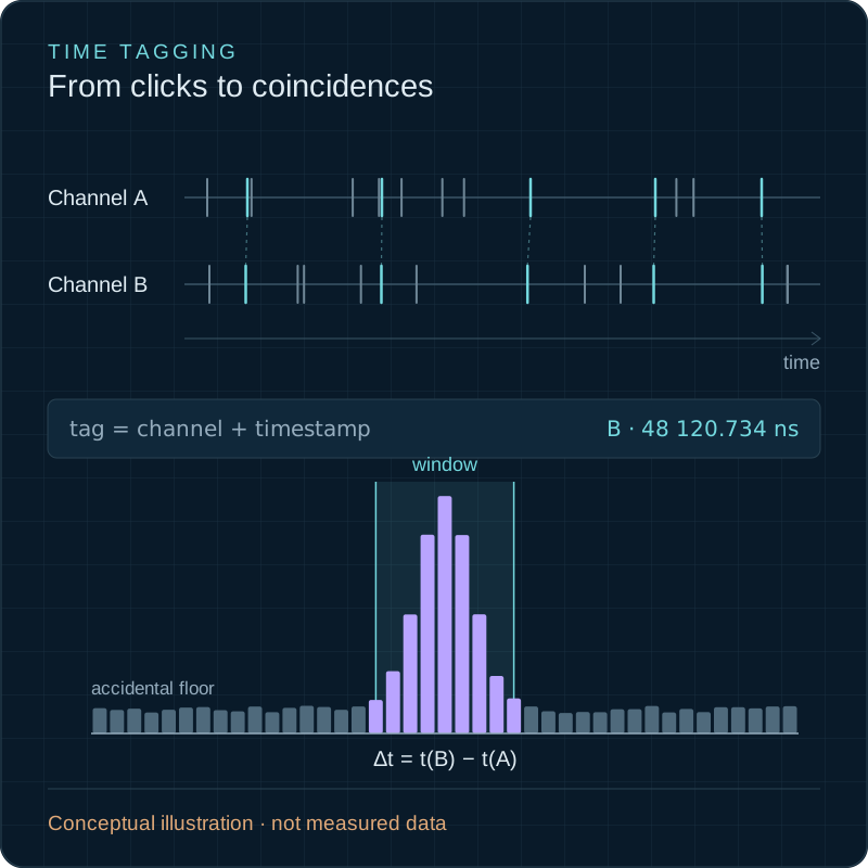
01 · Start with the experimental question
How do you know whether two detector clicks belong together?
A single-photon detector turns each detection into a short electrical pulse. The pulse says that something arrived, a photon or a dark count, but not whether it is related to a click on another detector. That is a question about timing.
A time tagger records the arrival time and the input channel of every pulse. Software can then compare the streams, histogram the differences between arrival times, and look for structure that unrelated events would not produce.
Photon
reaches the detector
Detector
turns a detection into a pulse
Electrical pulse
its edge crosses a threshold
Timestamp + channel
recorded for every event
Correlation histogram
of arrival-time differences, built in software
| Aspect | Counting events | Time tagging events |
|---|---|---|
| Records | How many pulses arrived in a gate or interval | When each pulse arrived, and on which channel |
| Answers | How bright is the source? Is the rate stable? | Which events occurred together, and at what delay? |
| After the run | Totals, and any coincidence window set in hardware, are fixed | Delays and windows can be changed and the data reanalysed |
A counter answers how many. Correlation measurements need when, which is what a time tagger keeps.
02 · Inside the instrument
How a time tagger works — and where the FPGA fits
The input electronics compare each detector pulse with a threshold and register the moment its edge crosses it. A time-to-digital converter (TDC) then measures that moment against a reference clock, typically by counting clock cycles and interpolating within one.
A field-programmable gate array (FPGA) is configurable digital hardware that can process many event streams in parallel. Depending on the architecture, the FPGA implements the TDC itself or works alongside separate timing circuitry. It attaches a channel number to each timestamp, merges and buffers the streams, and keeps every input on a common timebase. Where the instrument supports it, it can also filter events or count coincidences before the data leave the device.
Software on the computer builds histograms and analyses the recorded timestamps.
Signals in
- Detector pulses on channels 1…N
- Laser sync or reference clock, if used
Inside the time tagger
Input stage
- Threshold and edge detection
- One event per crossing
TDC
- Time of each edge against a reference clock
- Coarse count + fine interpolation
FPGA
- Channel + timestamp per event
- Merge, order, buffer
- Common timebase, sync
- Filtering or coincidences, where supported
Computer
- Histograms and g²(τ)
- Stored tags for reanalysis
Many events
Parallel hardware and buffers keep up with high and bursty count rates on several inputs at once.
Coordinated channels
All inputs share one timebase, so a delay between two channels is a number you can measure and correct.
Timestamps kept
Stored tags can be histogrammed again with a different delay or window, without repeating the experiment.
What the FPGA does not decide
Not every calculation happens inside it: histograms and correlation functions are often computed in software. Not every time tagger offers hardware coincidence logic or real-time feedback outputs. And the FPGA clock frequency alone does not set the timing resolution; interpolation within the clock period, calibration, input noise and the detectors do.
03 · Application A
SPDC photon-pair coincidence measurements
In spontaneous parametric down-conversion (SPDC), a pump photon in a nonlinear crystal occasionally splits into two lower-energy photons, called signal and idler. The two are created together, within a correlation time that is usually far shorter than the timing jitter of the detection system.
Swipe sideways to see the whole diagram.
What the researcher does
- 1Records timestamps from both detectors over the same acquisition.
- 2Plots a histogram of the arrival-time differences, t(B) − t(A).
- 3Finds the correlation peak, which sits at the cable and detector delay between the channels, and compensates that delay so the peak is centred at zero.
- 4Chooses a coincidence window W centred on the peak.
- 5Estimates the accidental coincidences, from the singles rates or from the flat background away from the peak, and evaluates the pair signal against them.
The window is a trade-off. Too narrow, and it cuts off correlated detections in the wings of the peak. Too wide, and it admits more accidental coincidences between unrelated photons, which grow in proportion to the window width.
A common practical use is heralding: a detection in the idler arm announces that a signal photon is on its way, which turns a pair source into a heralded single-photon source for a downstream experiment.
Estimating accidentals and the pair signal
Accidentals from the histogram, using bins well away from the peak:
N_acc ≈ (mean counts per bin off the peak) × (W / bin width)
Accidentals from the singles rates, as in the lab below (continuous-wave pumping, low occupancy):
N_acc ≈ R_A × R_B × W × T
Net pairs inside the window, the coincidence-to-accidental ratio, and the heralding efficiency of the signal arm (N_idler is the idler singles count over the same time):
N_pairs ≈ N_window − N_acc
CAR = N_pairs / N_acc
η_signal ≈ N_pairs / N_idler
Counts are Poisson distributed. When the background estimate uses many off-peak bins, the uncertainty of N_pairs is close to √N_window. Pulsed pumping changes the picture: accidentals then sit in side peaks spaced by the laser period, and multi-pair emission within one pulse contributes to the central peak.
04 · Application B
Testing a single-photon emitter with HBT
Take a single quantum dot, or a diamond colour centre such as the nitrogen-vacancy (NV) centre. In a Hanbury Brown–Twiss (HBT) measurement its emission is split by a 50:50 beam splitter onto two detectors, and the time tagger records the arrival-time difference τ between the two channels.
Swipe sideways to see the whole diagram.
A single emitter cannot send one photon to each detector at the same moment: after emitting, it has to be excited again. Coincidences near τ = 0 are therefore suppressed. That suppression is the antibunching dip in the normalized second-order correlation function, g²(τ).
A value of g²(0) below 0.5 is commonly used as evidence of predominantly single-photon emission under appropriate measurement conditions. Interpretation also depends on background light, the timing response, the normalization and the statistical uncertainty.
Swipe sideways to see the whole diagram.
Raw coincidence counts are not g²(τ). They scale with the count rates, the bin width and the acquisition time, and only become g²(τ) once normalized.
Normalization, the 0.5 threshold, background and timing response
Continuous-wave normalization. For C(τ) coincidences in a bin of width Δτ, singles rates R₁ and R₂ and acquisition time T:
g²(τ) ≈ C(τ) / (R₁ × R₂ × Δτ × T)
Uncorrelated light gives 1 at long delays. Some colour centres show bunching above 1 at intermediate delays, so normalize at delays long compared with every timescale of the emitter.
Pulsed normalization. g²(0) ≈ area of the central peak ÷ mean area of the side peaks.
Why 0.5. N identical, independent single-photon emitters give g²(0) = 1 − 1/N, so two give 0.5. A value below 0.5 cannot come from two or more such emitters.
Background. Uncorrelated background with signal fraction ρ = S / (S + B) raises the measured value:
g²_measured(τ) = 1 + ρ² × [g²(τ) − 1]
Even a perfect single-photon source then shows g²(0) = 1 − ρ². Report raw values, any background correction, and how ρ was obtained.
Timing response. The histogram is g²(τ) convolved with the combined timing response of both detection channels. When that response is not much shorter than the dip, which is set by the emitter lifetime and the excitation rate, the dip is partly filled in.
Uncertainty. A bin with C counts has a Poisson uncertainty of about √C; quote g²(0) with its uncertainty.
05 · Interactive
Coincidence Window Lab
Plan a continuous-wave SPDC measurement: enter the singles rates, a window width and an acquisition time to see the accidental coincidences to expect. Open the timing model to add the pair peak.
Coincidence Window Lab
Accidental coincidences for a CW SPDC source
A planning model for continuous-wave pumping. Enter the singles rates, the full window width and the acquisition time.
Every preset is an illustrative set of numbers, not the performance of any detector, source or instrument.
Accepted interval: −W/2 to +W/2 around the delay-corrected peak centre.
Estimated accidental rate 10 counts per second; 100 accidental counts expected in 10 seconds.
Estimated accidental rate
10 counts/s
R_acc ≈ R_A × R_B × W
- Expected accidental counts in T
- 100
- N_acc ≈ R_acc × T
- W in seconds
- 1 × 10⁻⁹ s
- Accepted interval
- ±0.5 ns
- around the corrected peak centre
- Events per window (A / B)
- 1 × 10⁻⁴ / 1 × 10⁻⁴
- should stay well below 0.1
Widening the window captures more of the pair peak, but also more accidental coincidences.
At W = 1 ns the window keeps 98.1 % of the illustrative pair peak and admits 10 accidental coincidences per second.
Expected counts per 0.05 ns histogram bin over T = 10 s. Illustrative model, not measured data. Hover over the plot, or focus it and use the arrow keys, to read individual bins.
Timing model: pair peak and total coincidence rate
Treats the delay-corrected pair peak as a centred Gaussian whose width is the combined timing response of both detectors, the electronics and the time tagger. The plot uses these two values even while this panel is closed.
Full width at half maximum of the measured peak.
Pairs detected on both channels, integrated over the whole peak.
- σ = FWHM / 2.355
- 0.212 ns
- Accepted true-pair fraction
- 98.1 %
- Accepted true-pair rate
- 9,815 counts/s
- Expected total coincidence rate
- 9,825 counts/s
- Expected total coincidences in T
- 98,247
- Coincidence-to-accidental ratio
- 981
Total rate = accepted pairs + accidentals. The coincidence-to-accidental ratio (CAR) is taken here as accepted pairs ÷ accidentals; published definitions vary.
Equations, assumptions and the worked check
Equations
- W[s] = W[ns] × 10⁻⁹
- accepted: −W/2 ≤ Δt − Δt₀ ≤ +W/2
- R_acc ≈ R_A × R_B × W
- N_acc ≈ R_acc × T
- σ = FWHM / (2√(2 ln 2)) ≈ FWHM / 2.355
- f = erf[W / (2√2 σ)]
- R_total ≈ f × R_pair + R_acc
Δt₀ is the peak centre after the channel delays have been compensated, so the window is centred on the peak.
Worked check
R_A = R_B = 100,000 counts/s, W = 1 ns = 10⁻⁹ s, T = 10 s: R_acc = 10⁵ × 10⁵ × 10⁻⁹ = 10 counts/s, and N_acc = 10 × 10 = 100 accidental counts. The Worked check preset reproduces it.
Assumptions
- Count rates are stationary over the acquisition.
- Low event occupancy: R_A × W and R_B × W are well below 1.
- Accidental events on the two channels are approximately independent.
- Saturation and dead time do not distort the rates or the histogram.
- The measured singles include the paired detections, which slightly overstates accidentals for a very efficient source.
This is not a universal pulsed-source model. With pulsed pumping, accidentals collect in side peaks at multiples of the laser period and multi-pair emission within one pulse adds to the central peak.
Planning a measurement with these numbers? Send them with your enquiry and add your detectors and channel count.
Send these numbers06 · Specifications
What specifications actually matter?
Each line below matters for what it does to the measurement. A smaller timestamp increment does not automatically produce a better measurement: the coincidence peak is as wide as the combined jitter of detectors, electronics and tagger.
| Specification | Experimental consequence | Ask for |
|---|---|---|
| Timestamp resolution vs actual timing jitter | Resolution is the digital increment of a timestamp. Jitter is the random spread of measured times. Jitter, not the increment, sets the width of a coincidence peak. | RMS jitter per channel and between two channels, and how it was measured |
| Detector jitter and total system timing response | Detector and electronics jitter add to the tagger’s. The total sets the window you need, the accidentals you accept, and how much an HBT dip is filled in. | Detector jitter at your count rate and bias; the combined response shape, including tails |
| Channel count, including sync or reference inputs | Pairs and HBT need two detectors; polarization analysis often four; pulsed work adds a laser sync. | How many inputs work at once, and whether sync inputs count against them |
| Per-channel and aggregate sustainable event rates | Bright SPDC sources can exceed what an input, or the link to the computer, sustains continuously even when short bursts are fine. | Sustained rate per channel, across all channels, and to the computer |
| Dead time, buffering, overflow reporting, data transfer | Events lost after a click or dropped when buffers fill bias both rates and correlations. Losses should be flagged, never silent. | Dead time per channel, buffer depth, how overflows appear in the data |
| Electrical input compatibility and trigger thresholds | Detector pulses differ in polarity, amplitude and rise time. Threshold and edge choice affect jitter and amplitude-dependent timing shifts (walk). | Input impedance and voltage range, adjustable threshold, edge selection |
| Clock stability and synchronization | Drift during a long acquisition broadens peaks. Several instruments, or separated setups, need a shared reference. | Reference clock input and output, stability, multi-unit synchronization |
| Timestamp access, software/API support and reanalysis | Raw timestamps let you change delays and windows after the run and look for artefacts. | Raw tag streaming, file formats, programming interfaces, offline analysis |
How timing contributions combine
For independent, roughly Gaussian contributions, the width of the coincidence peak adds in quadrature:
σ_peak² ≈ σ_detA² + σ_detB² + σ_tagA² + σ_tagB² · FWHM ≈ 2.355 σ
Illustrative numbers: two detectors at 40 ps RMS and two tagger channels at 10 ps RMS give σ_peak ≈ 58 ps (FWHM ≈ 137 ps). Cutting the tagger channels to 1 ps RMS only brings that to 57 ps.
The timestamp increment adds quantization noise of about increment ÷ √12 RMS, which is usually small next to detector jitter. Real detector responses are often not Gaussian: an exponential tail widens the base of the peak and calls for a wider window than the FWHM alone suggests.
07 · Your experiment
Planning a photon-pair or single-photon experiment?
Contact us — we have a solution for your quantum optics experiment. Tell us what you want to measure, and we can discuss a suitable timing approach.
Useful to include
- Your application: SPDC coincidences, heralding, HBT and g²(τ), or something else
- Detector models and the pulses they output
- Channel count, including sync or reference inputs
- Expected singles and pair or coincidence rates
- Timing requirements: peak width, coincidence window, resolution
- Continuous-wave or pulsed excitation, and the repetition rate
The contact form opens with these questions filled in; answer what you can.
Sources and further reading
- Hanbury Brown & Twiss, Correlation between photons in two coherent beams of light, Nature 177, 27–29 (1956).
- Burnham & Weinberg, Observation of simultaneity in parametric production of optical photon pairs, Physical Review Letters 25, 84 (1970).
- Kimble, Dagenais & Mandel, Photon antibunching in resonance fluorescence, Physical Review Letters 39, 691 (1977).
- Michler et al., A quantum dot single-photon turnstile device, Science 290, 2282–2285 (2000).
- Kurtsiefer, Mayer, Zarda & Weinfurter, Stable solid-state source of single photons, Physical Review Letters 85, 290 (2000).
- Brouri, Beveratos, Poizat & Grangier, Photon antibunching in the fluorescence of individual color centers in diamond, Optics Letters 25, 1294 (2000) — background correction of g²(τ).
- Kalisz, Review of methods for time interval measurements with picosecond resolution, Metrologia 41, 17–32 (2004).
- Hadfield, Single-photon detectors for optical quantum information applications, Nature Photonics 3, 696–705 (2009).
- Migdall, Polyakov, Fan & Bienfang (eds.), Single-Photon Generation and Detection, Academic Press (2013).


