It is a mode-matching problem
A bright spot on the core is not enough. Position, angle, size, phase curvature—and for PM fiber, polarization—must match the accepted mode.
Photonics · practical design guide · 24 min
Collimation, beam shaping, mode matching, alignment, polarization, and coupling-efficiency troubleshooting—from the emitting facet to a launch that stays aligned.
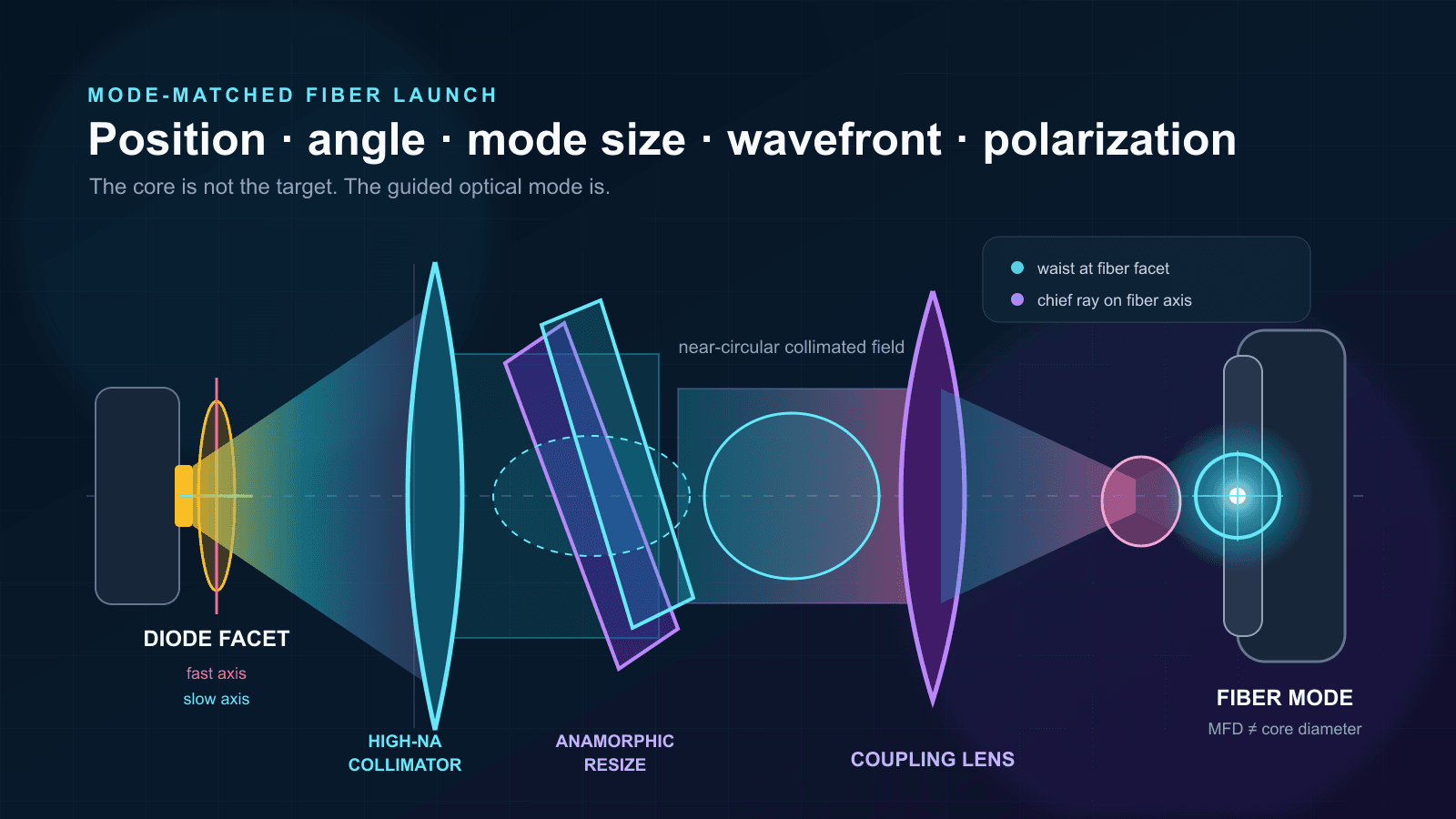
A bright spot on the core is not enough. Position, angle, size, phase curvature—and for PM fiber, polarization—must match the accepted mode.
Single-mode coupling is a complex-field overlap. Multimode coupling is governed by core, NA, launch phase space, and modal distribution.
Passive optics can resize or reject parts of a high-M² beam, but cannot transform all of it into a perfect Gaussian or increase source brightness.
1 · Start at the source
A diode’s emitting region is a thin, wide waveguide. The small vertical dimension diffracts strongly and defines the fast axis; the wider lateral dimension diverges less and defines the slow axis. The result is usually elliptical, linearly polarized, and different in amplitude and phase along the two axes.
The apparent waist positions can be separated along Z—astigmatism—and gain-guided or broad-area emitters can show lobes and non-Gaussian structure. M² must therefore be measured per principal axis. A value above 1 describes propagation departure from an ideal Gaussian, but does not contain enough phase information to predict exact fiber overlap by itself.
Wavelength, divergence, pointing, and polarization can move with drive current and junction temperature. A bare diode exposes all of this behavior. A collimated module hides some alignment but does not guarantee a circular, collimated, diffraction-limited field. Measure the delivered beam at the operating power and after thermal equilibrium.
The chip/package exposes the native divergent field. It needs a rated mount, current and TEC control, collimation, ESD protection, and feedback management.
Adds thermal and electrical interfaces, but may still expose the raw facet beam. Confirm whether a collimator or protective window is present.
Includes factory-set collimation. Measure the residual waist, divergence, ellipticity, astigmatism, and polarization rather than assuming a circular Gaussian.
The diode-to-fiber alignment is factory packaged. You design around pigtail fiber, connector, power, PER, stability, and bend limits.
A hermetic package commonly integrating a diode, TEC, thermistor, monitor photodiode, and fiber pigtail; pinout and controller compatibility remain package-specific.
Adds current/temperature control, interlocks, enclosure, and often monitoring. It minimizes optical integration but does not remove wavelength, noise, feedback, or fiber-compatibility checks.
2 · Define the requirement
A coupling target without wavelength, MFD or core, NA, stability interval, and polarization requirement is not specified. Use this as a design-review input sheet.
Wavelength and tolerance; power at the facet or module output; fast/slow full divergence with stated convention; M² in both axes; near-field structure; waist location; polarization and its drift.
Type; core diameter; NA; MFD at the operating wavelength; cutoff wavelength; cladding and coating; connector/polish; power handling; bend limits; PM axis and key convention.
Required delivered power and efficiency; output modal distribution; PER; drift over the relevant time; reconnect repeatability; allowable back-reflection.
Available working distance and beam height; required degrees of freedom; coarse capture range; fine sensitivity; stack height; stiffness; locking; left/right access; cable and thermal loads.
Warm-up, ambient range, airflow, vibration, cleanliness, enclosure, humidity, vacuum or magnetic constraints, and whether the assembly is adjustable or permanently packaged.
3 · Choose the fiber model
| Fiber | Coupling objective | Alignment | Polarization | Typical use | Main limitation |
|---|---|---|---|---|---|
| Single-mode (SM) | Maximize normalized field overlap with LP₀₁ at the facet. | Highest lateral, angular, focus, and wavefront sensitivity; tighter at small MFD and short wavelength. | Accepts two near-degenerate polarization states; ordinary SM fiber does not preserve an arbitrary input state under stress and temperature change. | Spatial filtering, interferometry, confocal excitation, coherent delivery. | MFD and cutoff are wavelength-dependent; core diameter is not the coupling target. |
| Multimode (MM) | Place the launch distribution inside the physical core and accepted angular phase space. | Usually more tolerant of lateral error; focus and angle still set which modes are excited. | Normally not polarization-maintaining; modal mixing can further alter the output state. | High-power delivery, illumination, pumping, collection. | High total power does not imply a stable near field, far field, or speckle pattern. |
| Polarization-maintaining (PM) | Match LP₀₁ and launch linear polarization onto one principal birefringent axis. | SM-level spatial sensitivity plus controlled fiber roll or polarization rotation. | Preserves an axis-aligned state; PER is limited by angular launch error, connectors, splices, stress, and the weakest component. | Raman, coherent detection, modulators, interferometers, polarization-sensitive experiments. | Maximum total power can occur while both axes are excited; measure PER as well as throughput. |
| Large-mode-area (LMA) | Launch into a larger guided mode while managing higher-order-mode content. | Larger mode may relax position tolerance, but bend, launch, and mode discrimination remain important. | Available in ordinary and PM designs; verify the actual construction. | Higher-power amplifiers, low-nonlinearity delivery, specialty lasers. | “Large core” does not guarantee effectively single-mode behavior; check V-number, bend design, wavelength, and launch. |
The target includes amplitude and phase. A spot with the correct diameter can still couple poorly if the wavefront curvature, angle, ellipticity, astigmatism, or lateral position is wrong. The accepted fundamental mode spatially filters everything else.
Core overlap and NA determine gross acceptance, but launch position, angle, focus, M², and bends decide which modes carry power. Underfill can improve output stability; overfill wastes power and can make connector heating worse.
4 · Collimate, then shape only if needed
The lens NA must cover the diode’s fast-axis half-angle at the stated beam-width convention. An NA label alone does not guarantee the clear aperture captures the displaced or astigmatic field.
For measured full divergence Θ, the first estimate of 1/e² collimated diameter is 2f tan(Θ/2). Short f produces a smaller beam and tighter lens-to-facet tolerance; long f produces a larger beam and more mechanical access.
The principal plane must reach the emitting facet without the barrel, mount, or window interfering. Packaged windows change the optical prescription.
A high-NA asphere often controls spherical aberration better than a singlet, but residual diode astigmatism and field structure remain.
Match the AR band, material, absorption, damage specification, and thermal lensing risk to wavelength, CW/peak power, and beam size.
Follow the lens drawing and manufacturer prescription. There is no universal “curved side toward the diode” rule that is safe across asphere designs and conjugates.
Measure beam width at multiple Z positions, separately along the fast and slow axes. Adjust lens-to-diode distance until the intended axis has minimal slope; if the other axis reaches its waist elsewhere, you have residual astigmatism, not a reason to average the two measurements. Also inspect for asymmetric clipping and structure that moves with aperture.
Fewest surfaces and stiffest mechanics. Start here when the unshaped overlap already meets the delivered-power and stability requirement.
Cost: Residual ellipticity and astigmatism may cap SM overlap.
Continuously resizes one axis and can circularize a modestly elliptical collimated beam.
Cost: Reflection loss, polarization-dependent transmission, beam walk, and two extra angular alignments.
Independent magnification or focus in one principal axis; useful for ellipticity and astigmatism correction.
Cost: Spacing, clocking, and decentration are sensitive; aberrations rise when used outside prescription.
Collimate fast and slow axes separately close to a high-divergence emitter or laser bar.
Cost: Very short working distance and packaging tolerances normally favor factory assembly.
Changes both axes together to match the coupling lens and target mode without changing ellipticity.
Cost: Adds length and surfaces; cannot repair axis-specific focus separation.
Rejects high-spatial-frequency structure and delivers a cleaner downstream mode.
Cost: Discarded power is the price; it cannot increase source radiance or recover brightness.
5 · Select the coupling optic
| Optic | Why use it | What to verify |
|---|---|---|
| Aspheric lens | Compact, high NA, short focal lengths, good access when mounted correctly. | Tight axial tolerance; verify conjugates, orientation, coating, clear aperture, and wavefront error. |
| Microscope objective | Convenient high NA and magnification choices; useful for exploratory lab coupling. | Correction collar, cover-glass design, field stop, back aperture, coating, and damage behavior may be unsuitable for the exact launch. |
| Fiber collimator | Connectorized and mechanically repeatable for a known wavelength/fiber family. | Usually designed to collimate fiber output; reverse use still requires wavelength, MFD, connector, return-loss, and power compatibility. |
| GRIN lens | Very compact, with a short packaged optical train. | Pitch, wavelength, facet spacing, centration, and aberration are design-specific. |
| Custom micro-optic | Best path to low size, weight, and alignment count in production. | NRE, tolerancing, metrology, and assembly yield dominate; not a fast laboratory fix. |
For an approximately collimated beam of 1/e² radius win, a thin lens of focal length f gives w0 ≈ M²λf/(πwin) in each principal axis. The approximation assumes a paraxial, separable field and ignores high-NA vector effects, lens aberration, truncation, residual curvature, and non-Gaussian diode structure.
Calculate fast and slow axes separately with their own win, M², and waist location. Then compare the focused 1/e² diameters with fiber MFD—not core diameter—for an SM/PM first pass.
6 · Coupling-efficiency physics
For incident complex field E and normalized guided mode F at the facet:
This captures amplitude and phase. It is the correct conceptual model even when the fields require measured wavefronts or numerical propagation.
For centred, coaxial, circular Gaussian modes with coincident waists and equal curvature:
Here w₁ and w₂ are 1/e² intensity radii; fiber MFD = 2w₂. This expression is not a multimode coupling formula.
A real measurement also includes Fresnel reflection at uncoated surfaces, absorption and scatter in every optic, connector and splice insertion loss, and loss from a dirty, scratched, or thermally damaged fiber facet. Keep those transmission terms separate from spatial overlap so an alignment problem is not “fixed” by silently renaming a connector loss.
Measured loss budget
Interactive first-pass estimator
Full divergence angles and beam diameters use the 1/e² intensity convention. For single-mode and PM fiber, the entered size is MFD; for multimode fiber it is physical core diameter.
Estimated delivered power
54.1 mW
The collimator NA covers both entered 1/e² divergence half-angles. Clear-aperture and working-distance checks still remain.
Collimated 1/e² diameters
2.9 × 0.8 mm
fast × slow, before shaping
Shaped beam diameters
2.9 × 2.4 mm
at the coupling optic
Estimated focused radii
1.6 µm × 2.5 µm
1/e² radii, fast × slow
Mode-size overlap
89%
target mode radius 2.6 µm
Polarization overlap
100%
cos² of PM-axis angle error
Total laser-to-fiber estimate
54%
includes nominal AR-optics transmission and collimator capture
Dominant estimated loss
Measure both M² axes and the near field. Passive optics can reshape the beam but cannot restore source brightness.
Stage configuration
Six-axis launcher; retain roll for PM-axis alignment.
Coarse acquisition comes before automated or piezo optimization.
Model assumptions
Separable Gaussian LP₀₁ approximation. The M² allowance is heuristic because M² does not uniquely specify the optical field.
Nominal transmissions are 96% per collimating/coupling optic and 94% for an active beam-shaping train. Connector, splice, contamination, aberration, and damage losses are not known and are excluded.
7 · Alignment hardware
Centre the focused field on the core or guided mode.
Usually the sharpest SM controls; use fine, low-backlash adjustment.
Place the waist and correct wavefront curvature at the facet.
Revisit after X/Y because lateral position and focus interact.
Align the chief ray and wavefront normal to the fiber axis.
Most useful for SM, small-MFD, long free-space paths, or when the pivot is near the facet.
Align linear polarization with the selected PM fast or slow axis.
A throughput peak is not enough; optimize the measured extinction ratio.
Dither, track drift, or recover a narrow optimum after coarse capture.
Needs a stable coarse stage, controller, sensor, travel margin, and feedback logic.
Put angular pivots near the fiber facet, keep stack height and the laser-to-fiber mechanical loop short, and choose sensitivity substantially finer than the optical tolerance. Evaluate backlash, stiffness, lock shift, cable force, thermal drift, load, handedness, and whether moving the fiber or moving the laser keeps the cleaner mechanical reference. A six-axis tower that flexes is not automatically better than a stiff five-axis stage.
UFP3C supplies XYZ for tolerant MM work; UFP5C adds two angular axes for SM; UFP6C adds roll for PM or full six-DOF alignment.
Verified: Repository catalog: ±6.5 mm coarse and ±0.3 mm fine linear travel, ≤0.5 µm fine sensitivity; micrometer-driven crossed-roller stages.
Limit / compatibility: They are manual—not motorized, piezo, or closed loop. Load rating falls from 1.5 kg (3-axis) to 0.5 kg (6-axis); choose left/right access deliberately.
Stainless XYZ, five-axis, and six-axis assemblies for sub-micrometre manual fiber and photonic-device alignment.
Verified: Repository catalog: 13 mm X/Y travel, 6 mm Z travel, <1 µm linear sensitivity, crossed-roller linear guidance, and dovetail angular modules.
Limit / compatibility: Manual micrometer actuation; the angular ranges and handed variants differ by module. Verify footprint, optical height, and access in CAD.
A stiff common-body platform when backlash, stacked-stage error, or active fine correction limits a stable SM/PM launch.
Verified: Repository catalog: 4 mm XYZ travel, >130 Hz resonant frequency and 1 kg load. NXP-3NP/6NP variants add 19 µm typical closed-loop piezo travel and 1 nm linear resolution; NXP-6NP lists 0.018 µrad angular resolution.
Limit / compatibility: The piezo travel is a fine range, not the acquisition range. NXP-M variants require separate DNXP manual or motorized drivers; do not infer closed loop from the flexure platform alone.
Build a replaceable launch module from dovetail fiber chucks, objective or GRIN holders, fixed stands, and XYZ/angular stages.
Verified: Repository catalog identifies <2 µm sensitivity for relevant APFP translation assemblies, an APFP-FH holder for nominal 125 µm bare fiber, and dedicated APFP-OM, APFP-GH, and APFP-FC carriers.
Limit / compatibility: Holder interfaces are specific: for example, APFP-OM uses a WJ 4/5-1/36″ objective thread and APFP-GH accepts optics below 4.8 mm diameter. Confirm the exact optic and chuck before ordering.
8 · Alignment workflow
Blindly scanning every axis is inefficient because most of the space contains no signal and several controls move the same spot. Establish position and angle first, search a bounded region, and reduce step size only after first light.
Confirm wavelength, divergence convention, M² axes, power, fiber MFD/core, NA, cutoff, connector polish, PM key, lens bands, and damage limits.
Use the correct mount, current driver, TEC, thermistor, ESD controls, and interlock. Let the complete mechanical loop warm up.
Use the lowest practical power, rated attenuation and enclosures. Establish instrumented viewing appropriate to the wavelength.
Set the manufacturer-prescribed orientation and working distance without contacting the package or facet.
Measure beam size at several axial planes. One axis can appear collimated while the other remains converging because of astigmatism.
Compare measured ellipticity/waist separation with the required mode overlap. Add one controlled correction only when its benefit exceeds loss and drift cost.
Use irises, cameras, a target, or beam-position sensor at two separated planes. Do not infer angle from a single spot.
Place the fiber face near the predicted focus and orient the stage so adjustment access and cable routing do not load the moving body.
For MM, search the core plane. For SM/PM, use a larger capture signal or camera if available, then scan X/Y near the predicted Z.
At fixed Z, bracket the peak from both directions. A genuine SM peak should be smooth and reproducible.
Sweep through the maximum; return to X/Y because moving through a tilted beam shifts the spot.
Change one angle at a time around a useful pivot, then re-centre. Angular motion without a common pivot produces lateral walk.
Rotate the fiber or input polarization to the specified axis while measuring output through an analyzer or polarimeter.
Use decreasing step sizes: X/Y → Z → tip/tilt → X/Y → PM roll. Stop when improvements are below measurement repeatability.
Record power at a defined plane before the launcher and after the fiber. Subtract known connector/splice loss only when comparing spatial coupling.
Tighten in small increments while watching power. If locking moves the stage, repair preload or clamp geometry rather than accepting the loss.
Log input-normalized transmission through warm-up, airflow, gentle cable motion, connector handling, and expected vibration.
Add a correctly rated isolator, APC interfaces, enclosure, monitoring detector, or piezo re-optimization when the stability test shows a need.
9 · Optimization methods
| Method | How it works | Use / caution |
|---|---|---|
| Manual hill climbing | Move one control in both directions, retain the improvement, and reduce step size. | Fast for a visible, isolated peak; vulnerable to operator bias and coupled axes. |
| Raster scan | Map a bounded X/Y or X/Z rectangle at fixed settings. | Reliable for acquisition, but slow and wasteful if the search window is too large. |
| Spiral search | Expand from a credible predicted centre until a threshold is crossed. | Efficient when the initial axis is good; can miss peaks if scale or centre is wrong. |
| Coordinate descent | Optimize X, Y, Z and angles sequentially and repeat. | Simple and robust for near-separable peaks; stalls when controls are strongly coupled. |
| Dither and lock | Apply small orthogonal modulations, demodulate the normalized power gradient, and servo to zero slope. | Tracks drift continuously; dither amplitude, detector bandwidth, and experiment sensitivity must be managed. |
| Gradient / model-based search | Estimate local derivatives or fit a response surface, then choose the next motion. | Efficient with good SNR and smooth response; false local maxima and backlash corrupt the model. |
| Camera or QPD assisted | Separate beam position and angle using one or two planes before maximizing fiber power. | Improves acquisition and diagnosis; position sensors do not directly measure modal overlap. |
Repeat from both approach directions, map a neighborhood, and test the candidate against small perturbations and time.
Divide delivered power by a pre-launch monitor where source drift matters; filter within detector bandwidth without erasing the gradient.
An optimizer can chase a speckle realization. Average over the relevant bend, time, or agitation state if the application measures the average.
Diode emission is often strongly linearly polarized, but mirrors and especially prism shapers can rotate phase or change s/p transmission. For PM fiber, identify the slow and fast axes, verify the actual connector-key convention, align with a wave plate or fiber roll, then measure PER. Ordinary SM fiber can rotate polarization with temperature, bends, and stress; use a polarization controller or PM architecture when the downstream experiment requires a state.
Maximum coupled power is not necessarily maximum power in the intended PM axis.
Flat fiber facets, FC/PC connectors, lenses, windows, and downstream optics can return coherent light to the diode and change power, linewidth, spectrum, or mode. Use a wavelength- and power-qualified Faraday isolator, FC/APC where the whole interface is compatible, AR or wedged optics, and index matching only where approved. Slightly tilt reflective components when the optical design allows it.
Monitor spectrum and power while commissioning, and use the diode-stabilization guide. Deliberately spoiling fiber coupling is not a primary feedback-control method.
Peak efficiency is only a commissioning datum. Test warm-up, room temperature, airflow, table vibration, cable movement, fiber bend, connector handling, source power, and diode temperature. Shorten and stiffen the mechanical loop, lower stack height, enclose the path, strain-relieve the cable, route fiber cleanly, and use stable lens mounts.
When passive changes do not meet the drift budget, add input-normalized monitoring and periodic or continuous piezo re-optimization.
Laser safety
Standard references verified against the IEC catalogue in August 2026. IEC lists IEC 60825-1:2014 as the base Part 1 publication and IEC TR 60825-14:2022 as the current user guide; always check the edition adopted in your jurisdiction.
10 · Troubleshooting
| Symptom | Most likely cause | Diagnostic test | Corrective action |
|---|---|---|---|
| No detectable fiber output | Wrong focus plane, gross lateral error, blocked/clipped beam, wrong wavelength fiber, dirty cap/facet, or detector range. | Verify free-space power and axis at two planes; inspect the facet only with a rated video inspection system; use a bounded coarse X/Y scan at several Z values. | Restore the reference axis, clean with an approved process, confirm detector and fiber band, then reacquire coarsely. |
| Coupling only at one end of stage travel | Mechanical origin or beam axis is offset; coupling optic is decentered. | Remove the fiber and project the focused axis relative to the launcher datum. | Re-centre the coarse mechanics before fine alignment; do not operate against a travel stop. |
| High coupling disappears when locked | Clamp force, backlash, or cable torque moves the fiber. | Watch normalized power while tightening each lock separately. | Correct preload and strain relief; lock incrementally from a repeatable approach direction. |
| Good at low power, poor at full power | Thermal lensing, diode pointing shift, mount heating, saturation/damage, or power-meter error. | Log beam position, spectrum, mount temperature, and input/output powers during a controlled ramp. | Improve thermal design or use power-rated optics/fiber; never realign through an active damage process. |
| Coupling changes during warm-up | Diode wavelength/pointing or mechanical loop is still drifting. | Normalize fiber power to a pickoff before the launcher and log temperature and position. | Allow full equilibrium, shorten the mechanical loop, enclose it, or add slow correction. |
| Output fluctuates when cable moves | Bend-dependent polarization or modal distribution; cable force reaches the stage. | Move only a downstream cable section while monitoring total power, PER, and near/far field. | Add strain relief and a stable route; use PM fiber or modal scrambling only when the application calls for it. |
| High PM throughput but poor PER | Both PM axes are excited or the connector/key/splice is misaligned. | Measure analyzer extrema or use a polarimeter while rotating roll. | Align the intended axis, verify key convention and splice orientation, and remove cable stress. |
| Strong back-reflection instability | Flat facet, FC/PC interface, window, or lens sends coherent feedback into the diode. | Monitor power and spectrum while introducing a rated isolator or changing a downstream reflection safely. | Use a suitable isolator, FC/APC, AR/wedged optics, and approved index matching where applicable. |
| Good coupling in one axis, poor in the other | Ellipticity, astigmatism, cylindrical-lens clocking, or clipping. | Measure both beam radii and waist positions through focus. | Correct only the limiting axis with lens spacing/magnification; check collimator fast-axis capture. |
| MM output changes when fiber bends | Launch distribution and mode coupling change with bend. | Compare total power, near field, far field, and speckle while applying the allowed bend range. | Stabilize routing and launch; use a mode scrambler only if averaged output is acceptable. |
| Coupling slowly decays over hours | Thermal creep, air flow, piezo drift, cable relaxation, or contamination. | Log normalized power, stage sensor, temperature, and beam position. | Remove the correlated disturbance, re-preload mechanics, enclose, or implement periodic correction. |
| Power plateaus at a low ceiling | Mode-size/wavefront mismatch, high M², clipping, aberration, polarization loss, or damaged facet. | Measure a full loss budget and map the near/far fields; compare with the unshaped path. | Change the optical architecture instead of searching more axes; accept the brightness-limited ceiling when appropriate. |
| Facet burns or contaminates | Power density exceeds condition or debris is heated at the facet. | Stop emission; inspect with a rated off-line fiber microscope and compare insertion loss. | Replace damaged fiber/optic, improve cleaning and caps, verify power and spot-size ratings, and eliminate hot-plug exposure. |
| Optimizer finds unstable local maxima | MM speckle, detector noise, backlash, coarse step size, or a drifting normalization signal. | Repeat scans from both directions and compare raw versus input-normalized power. | Filter appropriately, average over modal fluctuations, compensate backlash, constrain the search, and validate the final peak over time. |
11 · Worked architectures
Why it fits: It prioritizes a clean LP₀₁ mode and keeps the free-space train short.
Why it fits: It protects spectral and polarization performance central to a quantitative Raman measurement.
Why it fits: A geometrical core-and-NA design is physically appropriate; forcing a Gaussian SM model would be misleading.
Why it fits: Active motion is justified because measured drift, not theoretical peak efficiency, is the binding requirement.
Why it fits: Factory alignment removes fragile degrees of freedom and often wins on size, assembly time, and production yield.
12 · Build or buy
| Architecture | Choose it when | Advantage | Cost / limit |
|---|---|---|---|
| Build a free-space launcher | Research setup, changing fibers or wavelengths, access to intermediate planes, or a beam-shaping experiment. | Maximum flexibility and diagnostic access. | More surfaces, skill, alignment time, feedback paths, and environmental drift. |
| Buy a pre-aligned fiber-coupled diode | Compact OEM, repeated builds, field use, or when alignment is not the research question. | Factory-set launch, small footprint, lower assembly variance. | Fixed fiber/connector, supplier dependence, limited repairability, and fewer optical degrees of freedom. |
| Use a replaceable coupling module | A platform needs serviceable source/fiber variants without rebuilding the base instrument. | Swap a qualified launch cartridge while retaining coarse datum and cable management. | Module repeatability and interface tolerance become system specifications. |
| Use an actively stabilized launcher | Measured drift exceeds the experiment budget and passive improvements are insufficient. | Recovers coupling and can log alignment state. | Sensors, controller, piezo travel, false maxima, dither, software, and failure handling add real complexity. |
Primary and manufacturer references
The calculator deliberately exposes its assumptions. Final lens orientation, wavelength band, damage limit, fiber MFD/NA/cutoff, connector keying, isolator performance, and stage configuration must come from the current item-specific datasheet.
Current base classification and product requirements; IEC lists stability through 2027 and incorporates the 2017 interpretation sheets.
User-oriented risk assessment and control-measure guidance.
Manufacturer technical reference for diode geometry, fast/slow divergence, astigmatism, and collimation.
Manufacturer reference for selecting a launch lens from wavelength, beam diameter, and MFD.
Fiber-manufacturer explanation of MFD, its wavelength dependence, and why it is not simply core diameter.
Manufacturer technical note on M² measurement, beam parameter product, and cylindrical correction of elliptical beams.
FAQ
The emitting junction is much thinner in one direction than the other, so diffraction is stronger on the fast axis. Different effective source positions and gain guiding can also create astigmatism and non-Gaussian structure.
Not universally. A suitable high-NA asphere is a strong compact starting point for many bare diodes, but a microscope objective, GRIN lens, factory collimator, or custom micro-optic may be better. The prescription, conjugates, coating, clear aperture, and working distance decide.
First ensure the NA captures the required divergence. Then use 2f tan(Θ/2) to estimate the collimated 1/e² diameter from measured full divergence Θ, and choose a diameter that the shaping and coupling optics can use without clipping.
The normalized overlap of the incident complex field with the guided fundamental mode. Mode size, ellipticity, phase curvature, position, angle, focus, polarization, aberration, clipping, facet condition, and source field quality all matter.
Some power can couple if the source has overlap with LP₀₁, but passive optics cannot compress all of a high-étendue, high-M² field into one diffraction-limited mode. The fiber rejects the rest, so efficiency can be intrinsically limited.
XYZ is often enough for MM acquisition. SM commonly benefits from XYZ plus tip/tilt. PM additionally needs controlled roll unless polarization is rotated elsewhere. Add axes only when their tolerances are in the measured error budget.
Core diameter is a physical glass-geometry dimension. MFD describes the transverse extent of a guided mode and commonly exceeds the core diameter; it changes with wavelength and may be defined by a standardized measurement rather than a simple Gaussian fit.
Launch a clean linear state onto the specified slow or fast axis by rotating fiber roll or the input polarization, then measure extinction ratio at the output. Confirm the connector-key convention from the actual cable datasheet.
Cable motion can torque the launcher, change micro/macro-bend loss, mix modes in MM fiber, or change polarization in ordinary SM fiber. Strain-relieve the cable and separate motion at the stage from changes in the delivered mode.
Diode pointing, wavelength, package stress, and the surrounding mounts can all move during thermal equilibrium. Normalize fiber power to a pre-launch pickoff to separate source-power drift from coupling drift.
FC/APC usually provides lower back-reflection at a mated interface, which is valuable for feedback-sensitive diode lasers, but every component and mating sleeve must be APC-compatible and keyed correctly. FC/PC remains useful where angular-polish geometry or compatibility makes APC unsuitable. Never mate PC to APC.
Use one when the diode is sensitive to feedback and the measured or credible return path exceeds its tolerance. Choose wavelength, aperture, isolation, insertion loss, polarization dependence, power, and beam size from a current datasheet.
Use motorized coarse acquisition or a bounded search to find the peak, then piezo dither/lock or coordinate correction with an input-normalized power signal. Add limits, noise filtering, backlash handling, and a recovery search.
A lock or clamp is changing preload and moving the controlled body. Approach from a consistent direction, monitor power during small tightening steps, reduce cable torque, and repair the clamp geometry if the shift is systematic.
Usually for compact, repeatable, or production systems; usually not when you must change fiber, access the free-space beam, study beam shaping, or service individual optics. Compare lifetime integration cost and stability, not only component price.
Continue designing
Separate thermal, current, feedback, and pointing drift.
Choose control, scrambling, or PM preservation.
Read beam quality, noise, linewidth, and stability correctly.
Match travel, resolution, load, and environment.
Engineering enquiry
We can help turn them into a collimation, launch-stage, polarization, feedback, and monitoring architecture—with the incompatibilities stated before hardware is selected.