Start with the sample
What changed across your graphene?
Growth, transfer and processing can affect different parts of a flake. Decide whether you need to compare layers, defects or peak shifts before setting up the map.
Save a spectrum at each point, with references for the interior, edge and bare substrate. Keep the spectra behind the colour map.
For the scattering basics, see our Raman microscopy guide.
Start with D, G and 2D
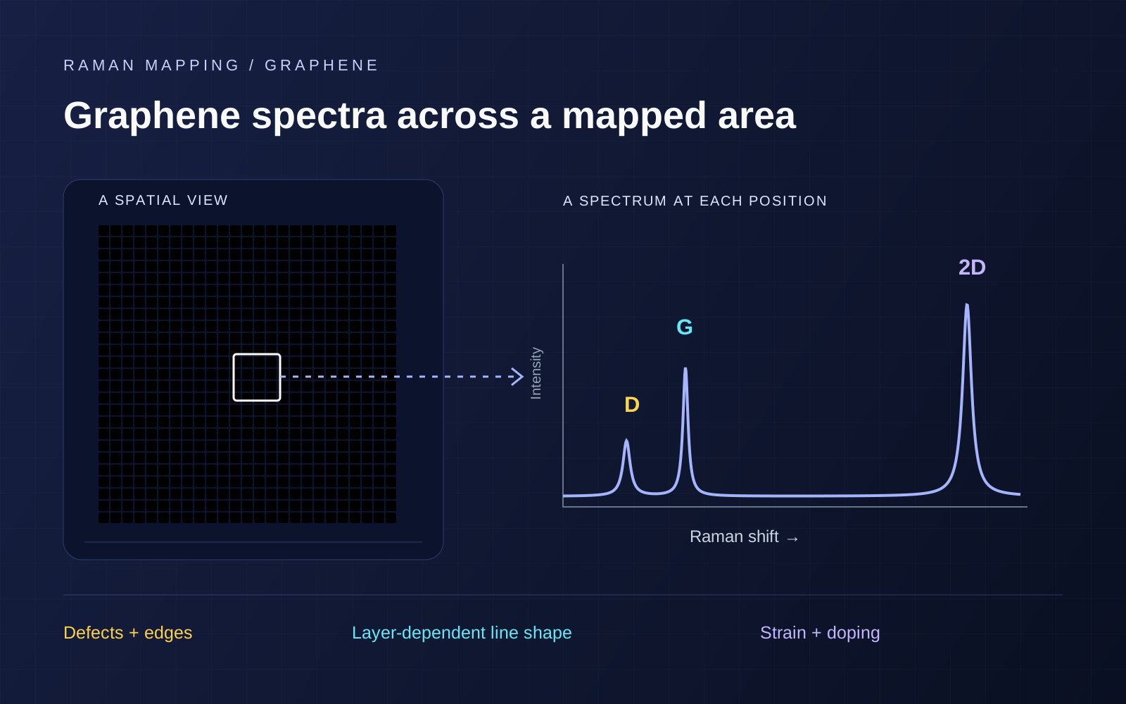
The approximate visible-excitation band positions are shown below. They shift with excitation and sample state. [1]
| Band | Record | Interpret with |
|---|---|---|
| D · ~1350 cm⁻¹ | D/G ratio and its location within the flake. | Edges, defect regime, excitation and polarization. |
| G · ~1580 cm⁻¹ | Position, linewidth and intensity. | 2D position, power dependence and fit quality. |
| 2D · ~2700 cm⁻¹ | Line shape, width, position and intensity relative to G. | A suitable layer reference, substrate and charge state. |
Label ratios as peak heights, I, or integrated areas, A. Width changes can make the two ratios differ.
Layers and defects
Layers: inspect the whole 2D profile
Compare the 2D profile with monolayer and few-layer references at matched excitation. Its shape and width carry layer information. [1]
Record the substrate stack: SiO₂/Si interference can change 2D/G intensity ratios. [2]
Defects: compare the boundary with the interior
Compare edge and interior spectra. Edges can produce D scattering, with a polarization-dependent response. [3]
D/G depends on excitation and can rise, then fall, with disorder. Establish the defect regime before converting it to density. [4]
Strain and doping
Plot fitted 2D frequency against G frequency. Their correlation helps separate strain and doping contributions. [5]
The tool compares representative strain and hole-doping directions. Quantitative analysis needs a reference and a model for the actual strain configuration, including shear or splitting where relevant. [6]
Interactive / G–2D correlation
Compare strain and hole doping
Compare G–2D shifts from strain and hole doping. Values are spectral contributions in cm⁻¹, not strain percentages or carrier densities.
Combined illustrative shifts
- ΔωG
- +3.0 cm⁻¹
- Δω2D
- -2.4 cm⁻¹
Model: ΔωG = S + H; Δω2D = 2.2S + 0.7H. The same +4 cm⁻¹ G shift gives +8.8 cm⁻¹ in 2D along the strain direction, versus +2.8 cm⁻¹ along the hole-doping direction.
Calculation and assumptions
Representative directions from Lee et al.; this simplified forward model omits electron doping, temperature, shear splitting and uncertainty. Real quantitative analysis needs the appropriate excitation, reference, strain configuration and calibration. See Mueller et al. for a treatment of arbitrary strain configurations.
Before the full map
Run a small pilot region first. Check these six things before committing to a long map.
- 01
Register the region.
Save the flake image, interior, edge and substrate positions, plus transfer history.
- 02
Choose and document the excitation.
Both featured systems offer 532 nm. Keep references matched when comparing excitation lines.
- 03
Check power and time dependence.
Vary power at the sample and repeat a spectrum. Watch for peak drift, background changes or a growing D band.
- 04
Calibrate and choose the spectral window.
Calibrate wavenumber. Confirm D, G and 2D fit in one detector window, or plan calibrated multiple windows.
- 05
Keep focus and acquisition settings consistent.
Keep objective, NA, pinhole, polarization and exposure settings consistent. Check focus across the area.
- 06
Fit, inspect and mask.
Review baselines, residuals and cosmic rays. Mask failed fits; don’t assign them zero defect density or shift.
See excitation wavelengths and spectrograph selection for more detail.
Example map
Graphene mapping with RTS-mini
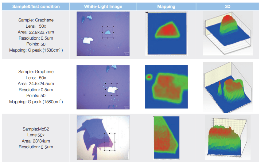
Sampling and map time
Choose spacing to sample the optical response. Smaller steps make a denser map; they do not improve optical resolution.
Measure exposure, motion and readout overhead on the pilot region. Include each spectral window and occasional reference checks in the time budget.
Interactive / Map-time planner
Estimate map time
Compare spacing, exposure and spectral windows. The grid includes both boundaries; halving spacing increases the point count in both directions.
Illustrative acquisition budget
15 min 48 s
- Grid
- 21 × 21
- Spectrum positions
- 441
- Actual X / Y spacing
- 0.500 / 0.500 µm
- Exposure subtotal
- 14 min 42 s
Both map boundaries are included. If a span is not divisible by your maximum spacing, this planner reduces the actual interval to fit that span.
Calculation and assumptions
Budget = positions × (exposure × accumulations × spectral windows + combined extra time per position). Enter a measured allowance for stage movement, readout, focus and window changes. A real system may use another scan mode or grid convention. This is a planning estimate, not an instrument speed specification; startup, calibration and unentered delays are excluded.
Which maps should you save?
G intensity
Locate signal and inspect illumination or focus variation. Brightness alone does not specify thickness.
D/G with an edge mask
Compare the boundary and interior while keeping excitation, polarization and intensity definitions fixed.
2D width and line shape
Compare layer-related spectral variation against the selected reference; inspect representative spectra behind each region.
G–2D positions and fit quality
Inspect correlated shifts alongside linewidths, residuals and uncertainty before assigning a material parameter.
Specify the shift you need to distinguish and its reference. Peak-fitting precision, spectral resolution and absolute wavenumber accuracy are different quantities.
Finder 930 or RTS-mini?
Choose a dedicated platform or add Raman to your microscope. Both need the right laser, spectral windows and mapping stage.
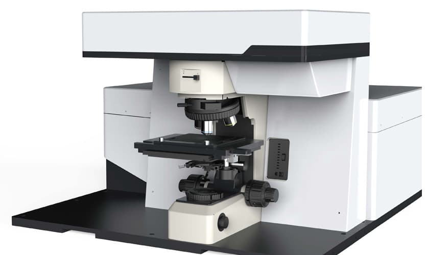
Build a dedicated mapping platform
Finder 930
A dedicated confocal platform for repeated maps. Choose the motorised mapping option and laser configuration for your samples.
- Excitation options
- 532 nm + 638 / 785 nm
- Published spectral resolution
- < 1.5 cm⁻¹
- Stage configuration
- Manual standard; motorised mapping option
The published <500 nm lateral-resolution figure is tied to 532 nm and a 50 µm pinhole; confirm the selected objective and configuration.
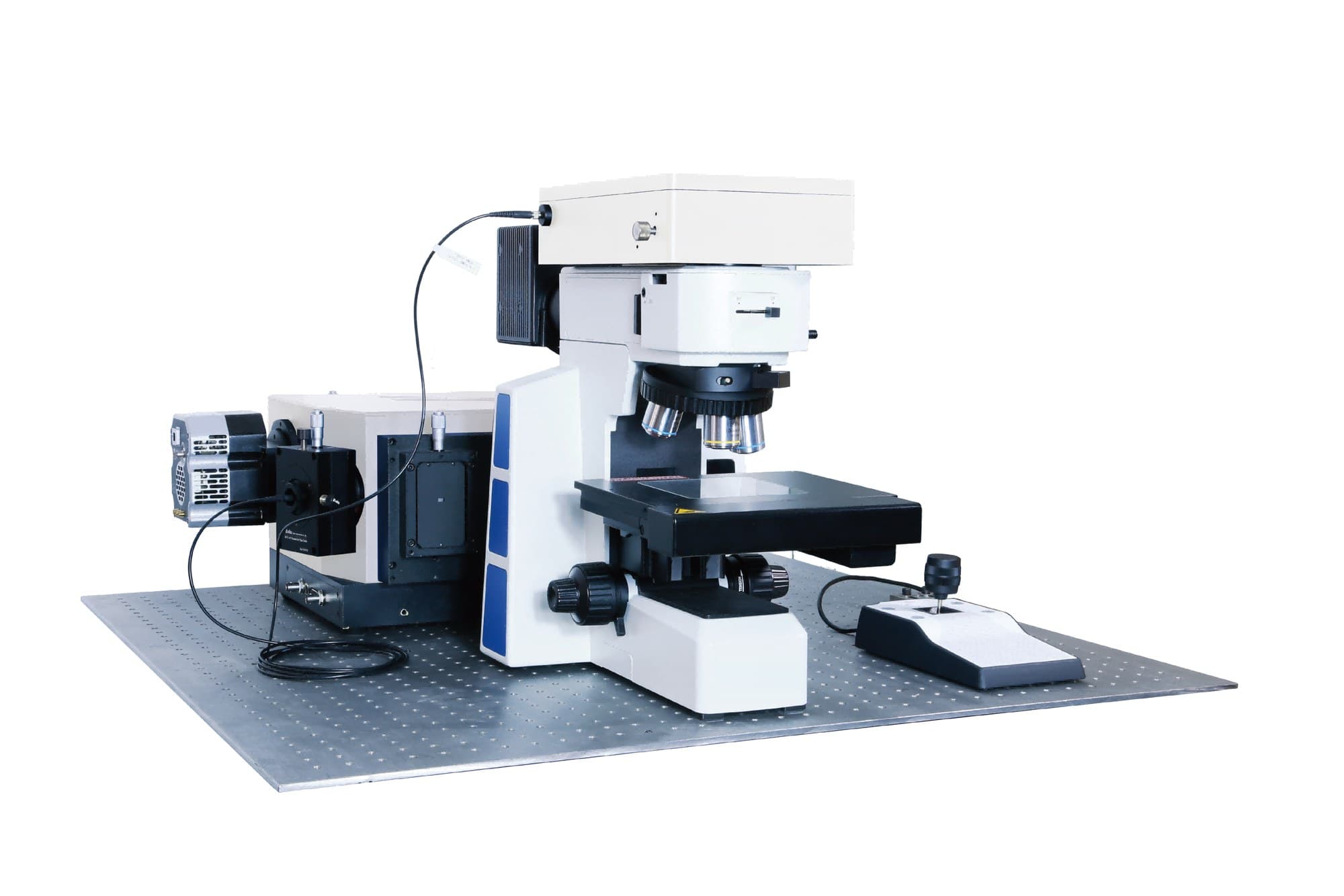
Add Raman to your upright microscope
RTS-mini
Add confocal Raman to a compatible upright microscope. Include motorised mapping and confirm objective and sample clearance.
- Excitation options
- 532 / 638 / 785 nm
- Published spectral resolution
- 1.5 cm⁻¹ (532 / 638 nm)
- Stage configuration
- Manual standard; motorised stage optional
The catalogue gives 1.5 cm⁻¹ at 532 / 638 nm and 2.3 cm⁻¹ at 785 nm; confirm the selected grating and spectral window.
Ask us to confirm D/G/2D window coverage, calibration and timing. Browse the full Raman range for other sample formats.
From research question to configuration
Plan your graphene measurement
Send a sample image or spectrum, substrate, map area and the change you need to measure. Tell us which microscope you already use.
Discuss graphene mapping & request a quoteQuestions before your first map
Does a high 2D/G ratio prove monolayer graphene?
Compare the 2D shape and width with a reference. Substrate interference and charge state can change the ratio.
Does a D peak mean the whole flake is damaged?
An edge can activate D scattering. Compare boundary and interior spectra, accounting for polarization and spot overlap.
Does a 50 nm stage step give 50 nm Raman resolution?
No. It samples the optical response more densely. Optical resolution depends on the illumination and collection optics.
Which system should I start with?
Finder 930 for a dedicated confocal platform; RTS-mini for a compatible upright microscope. Include the motorised mapping option.
References and datasheets
- [1]Raman spectrum of graphene and graphene layers
Ferrari et al. (2006), Physical Review Letters 97, 187401. Layer-dependent 2D-band shape, width and electronic structure.
- [2]Interference effect on Raman spectrum of graphene on SiO₂/Si
Yoon et al. (2009), Physical Review B 80, 125422. The substrate can change the observed 2D/G intensity ratio.
- [3]Raman spectroscopy of graphene edges
Casiraghi et al. (2009), Nano Letters 9, 1433–1441. Edge-localised D scattering and polarization dependence.
- [4]Quantifying defects in graphene via Raman spectroscopy at different excitation energies
Cançado et al. (2011), Physical Review Letters 107, 186104. Excitation dependence and the non-monotonic D/G response to defect density.
- [5]Optical separation of mechanical strain from charge doping in graphene
Lee et al. (2012), Nature Communications 3, 1024. G–2D correlation analysis and representative strain / hole-doping directions.
- [6]Evaluating arbitrary strain configurations and doping in graphene with Raman spectroscopy
Mueller et al., 2D Materials 5, 015016 (2018; published online 2017). Hydrostatic and shear strain, peak splitting and the limits of a simple correlation model.
Instrument specifications are linked in the product cards. The hero and interactive plots are illustrations; the application map is supplier data.