How a single micron-sized bead, held in a beam of light, measures the viscosity and viscoelasticity of a microliter of sample. Scroll through the theory, play with the live simulations, and follow a worked application note — with references throughout.
The idea in one paragraph
Classical rheometers shear millilitres of sample between centimetre-scale plates. Microrheology replaces that machinery with a probe particle a few hundred nanometres across and asks a simpler question: how does this bead move? In a thin, watery fluid it diffuses freely; in a structured or elastic medium its motion is hindered and constrained.
Optical tweezers add control on top of observation. By trapping the bead in light we can calibrate forces to the piconewton, confine the particle to a known region, and — if we wish — drive it on demand. The result is a full viscoelastic characterisation from microliter volumes, without mechanical contact.
Near-infrared light is chosen because water and biological material absorb it weakly, minimising heating and photodamage in delicate samples. [6]
The physics
Everything downstream — viscosity, elasticity, frequency response — follows from these four foundations.
Every micron-sized particle suspended in a fluid is ceaselessly kicked by the molecules around it. The statistics of that jiggling encode the local mechanical properties of the medium.
A tightly focused laser creates a gradient force that pulls a dielectric bead toward the focus. For small displacements the force is linear, F = −k·x — a Hookean spring with stiffness k in the pN/µm range.
In equilibrium each degree of freedom carries ½kᴮT of energy, so ½k⟨x²⟩ = ½kᴮT. Measuring the variance of a trapped bead's position therefore calibrates the trap: k = kᴮT / ⟨x²⟩.
The generalized Stokes–Einstein relation converts the bead's mean-squared displacement into the complex shear modulus G*(ω) = G′(ω) + iG″(ω), giving elasticity and viscosity across frequency.
This is a real-time integration of the overdamped Langevin equation, γ ẋ = −kx + √(2γkᴮT)·ξ(t). Change the trap stiffness, the medium viscosity and the bead size, then watch how the position histogram and the recovered values respond. Notice that k and η are measured back out of the motion — exactly what the instrument does.
Turn the trap off to watch free Brownian motion — the bead wanders away. Turn it on and the same thermal kicks are now balanced by a spring-like restoring force, so the bead rattles inside a well whose width encodes the stiffness. The measured k and η are recovered purely from the recorded motion.
Model & calibration relations after Neuman & Block [6] and Berg-Sørensen & Flyvbjerg [7]. Units inside the solver: nm, ms, pN (kᴮT = 4.11 pN·nm at 25 °C).
Two modes of measurement
You can simply listento the bead's thermal motion, or actively drive it and measure the response. Both routes lead to the same viscoelastic moduli over complementary ranges.
The mean-squared displacement (MSD), ⟨Δr²(τ)⟩, is the central observable of passive microrheology. Its slope on a log–log plot is a fingerprint of the material: slope 1 for a simple liquid, a reduced slope for a viscoelastic solution, and a plateau for an elastic gel. Toggle the optical-trap confinement to see how the trap adds its own long-time plateau at ⟨Δr²⟩ ≈ 2kᴮT/k.
MSD scaling and interpretation after Squires & Mason [5] and Waigh [10].
The generalized Stokes–Einstein relation turns a measured MSD into the frequency-dependent storage modulus G′(ω) (elastic) and loss modulus G″(ω) (viscous). Here the moduli are computed live from a power-law MSD, ⟨Δr²⟩ = A·τα, using Mason's algebraic form |G*| = kᴮT / (πa·⟨Δr²(1/ω)⟩·Γ(1+α)).
Push α toward 1 and the response is dominated by G″ — a viscous liquid. Push α toward 0 and G′ rises above G″ — an elastic solid. The whole frequency spectrum here is computed from a single measured MSD curve through the generalized Stokes–Einstein relation (Mason 2000).
Algebraic GSER estimator after Mason [4]; underlying theory Mason & Weitz [3].
A representative workflow: characterising a dilute hyaluronic-acid (HA) solution — the kind of shear-thinning, viscoelastic fluid found in ophthalmic and dermal products — from a single 20 µL droplet. Numbers below are illustrative and typical of the method, not a validated product specification.
Good-practice notes. Keep the trap weak enough that the bead samples the material rather than the trap; hold temperature stable (viscosity of water changes ~2 %/°C); trap far from walls to avoid Faxén hydrodynamic corrections; and average several beads to separate local heterogeneity from measurement noise. See Squires & Mason [5] and Waigh [10] for the full caveats.
Why microrheology
| Property | Bulk rheometer | Optical-tweezers microrheology |
|---|---|---|
| Sample volume | 0.5–20 mL | 1–20 µL |
| Probe scale | mm–cm geometry | ~0.5 µm bead |
| Frequency range | ~10⁻² – 10² Hz | ~10⁻¹ – 10³ Hz |
| Contact | Mechanical shear | Non-contact, optical |
| Spatial resolution | Bulk average | Local, spatially resolved |
| Delicate samples | May disrupt structure | Gentle, non-invasive |
A. Einstein, “Über die von der molekularkinetischen Theorie der Wärme geforderte Bewegung von in ruhenden Flüssigkeiten suspendierten Teilchen,” Annalen der Physik 322(8), 549–560 (1905).
doi.org/10.1002/andp.19053220806A. Ashkin, J. M. Dziedzic, J. E. Bjorkholm, S. Chu, “Observation of a single-beam gradient force optical trap for dielectric particles,” Optics Letters 11(5), 288–290 (1986).
doi.org/10.1364/OL.11.000288T. G. Mason, D. A. Weitz, “Optical measurements of frequency-dependent linear viscoelastic moduli of complex fluids,” Physical Review Letters 74(7), 1250–1253 (1995).
doi.org/10.1103/PhysRevLett.74.1250T. G. Mason, “Estimating the viscoelastic moduli of complex fluids using the generalized Stokes–Einstein equation,” Rheologica Acta 39, 371–378 (2000).
doi.org/10.1007/s003970000094T. M. Squires, T. G. Mason, “Fluid mechanics of microrheology,” Annual Review of Fluid Mechanics 42, 413–438 (2010).
doi.org/10.1146/annurev-fluid-121108-145608K. C. Neuman, S. M. Block, “Optical trapping,” Review of Scientific Instruments 75(9), 2787–2809 (2004).
doi.org/10.1063/1.1785844K. Berg-Sørensen, H. Flyvbjerg, “Power spectrum analysis for optical tweezers,” Review of Scientific Instruments 75(3), 594–612 (2004).
doi.org/10.1063/1.1645654D. Mizuno, C. Tardin, C. F. Schmidt, F. C. MacKintosh, “Nonequilibrium mechanics of active cytoskeletal networks,” Science 315(5810), 370–373 (2007).
doi.org/10.1126/science.1134404F. Gittes, B. Schnurr, P. D. Olmsted, F. C. MacKintosh, C. F. Schmidt, “Microscopic viscoelasticity: shear moduli of soft materials determined from thermal fluctuations,” Physical Review Letters 79(17), 3286–3289 (1997).
doi.org/10.1103/PhysRevLett.79.3286T. A. Waigh, “Advances in the microrheology of complex fluids,” Reports on Progress in Physics 79(7), 074601 (2016).
doi.org/10.1088/0034-4885/79/7/074601The Nobel Prize in Physics 2018 — Arthur Ashkin, “for the optical tweezers and their application to biological systems.” NobelPrize.org.
www.nobelprize.org/prizes/physics/2018/summary/This note is educational. Simulations use simplified, quantitatively representative models; instrument performance figures are indicative and should be confirmed for your specific sample.
Before you specify
The trap, the mechanics, the detection chain, and the laser specifications that decide how gently you can hold a bead.
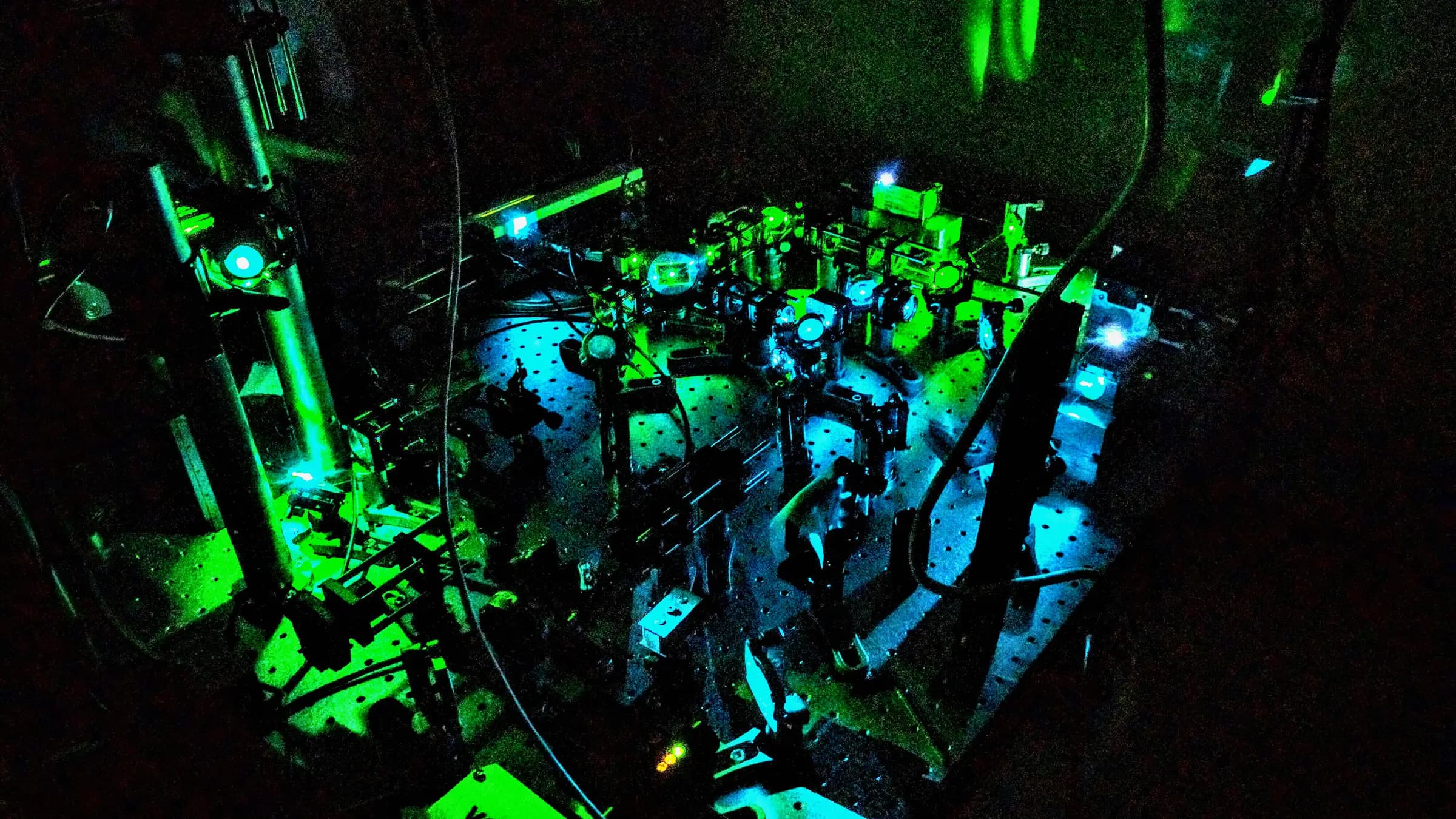
Optical microscopyDesign the trapping beam, objective, mechanics, imaging, QPD detection, calibration, and safety workflow as one instrument.
Open guide
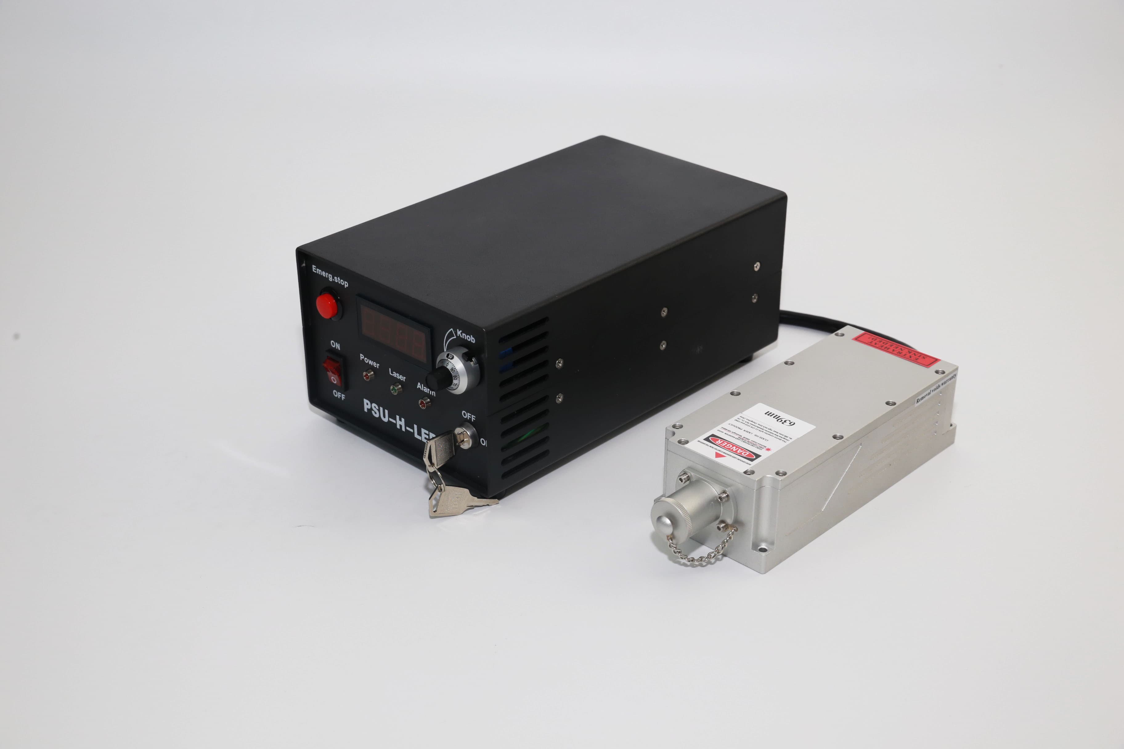
Optical trappingWhy wavelength is decided by photodamage, focal heating, and detector bandwidth rather than trapping force — and what laser noise costs you in piconewtons.
Open guide