Cells and biomaterials
Map acoustic contrast in cells, hydrogels and tissue; study spatial heterogeneity or responses to a controlled perturbation. Correlative fluorescence or chemical imaging helps identify the structures involved. [3][4]
Spectroscopy & optical mechanics
A practical guide to the physics, the instrument and the meaning of a mechanical contrast map.
A small frequency shift in scattered light carries information about acoustic waves inside a material. Measuring it takes a clean laser, strong rejection of elastic scattering and a carefully calibrated spectrometer. Interpreting it requires equal care with the material model.
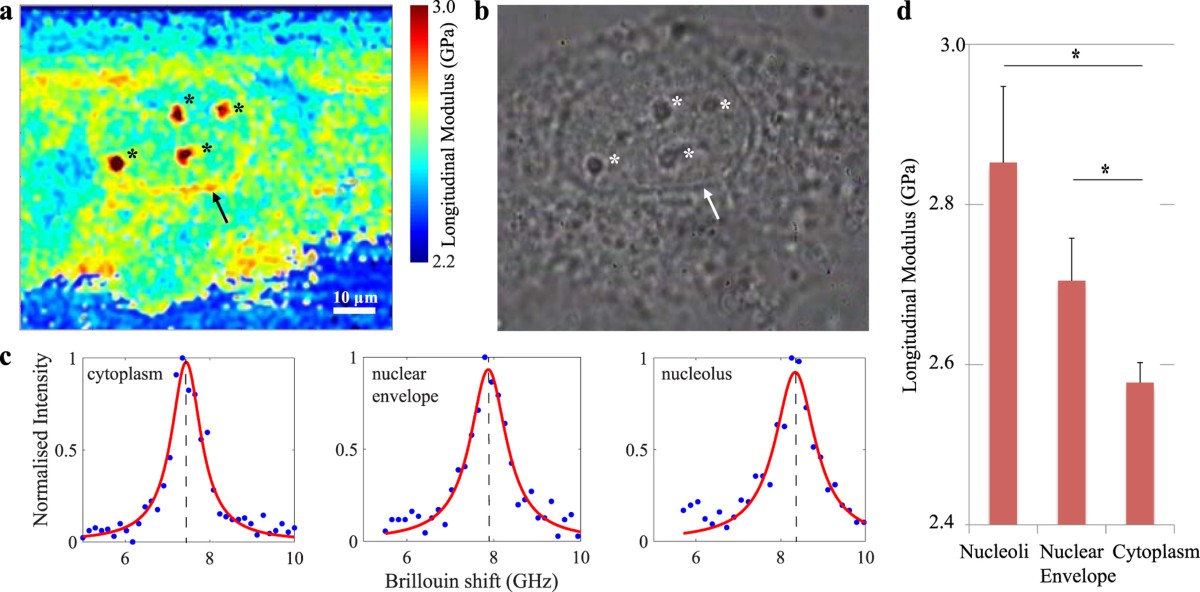
Published cell data: a Brillouin map, phase-contrast image and fitted spectra from different cellular regions. The colour scale reports the authors’ derived longitudinal modulus, not Young’s modulus.
Figure 2 from Biomechanics of subcellular structures by non-invasive Brillouin microscopy. Giuseppe Antonacci and Sietse Braakman. Scientific Reports 6, 37217 (2016). © The Author(s) 2016. DOI / source. Reproduced under CC BY 4.0. Complete figure; no content changes. Display size and image encoding may differ.
Open full-size figure ↗01 / Brillouin spectroscopy
Brillouin light scattering is inelastic scattering from acoustic excitations. In a spontaneous experiment, thermal density fluctuations scatter a small fraction of the incident light. The Stokes component loses energy to the material; the anti-Stokes component gains energy. They appear on opposite sides of the much stronger, unshifted elastic line. [1][3]
In an isotropic, transparent bulk material, the scattering geometry selects an acoustic wavevector. The frequency shift then gives the corresponding sound speed. Changing angle changes the acoustic mode sampled; measurements from different geometries cannot be compared solely by comparing their peak positions. [1][9]
Bulk longitudinal mode · weak damping
fB = (2nvL / λ0) sin(θ / 2)
M′ ≈ ρ [λ0fB / (2n sin(θ / 2))]²
Here fB is ordinary frequency in Hz, λ0 is the vacuum wavelength, n the refractive index, ρ the mass density and θ the scattering angle inside the sample. Backscattering has θ = 180°.
For illustrative water-like inputs n = 1.333, vL = 1,480 m/s, ρ = 998 kg/m³ and 532 nm backscattering, fB ≈ 7.42 GHz and M′ ≈ 2.19 GPa.
That shift is about 0.247 cm⁻¹, or 0.0070 nm at 532 nm. A conventional Raman spectrograph specified at 1 cm⁻¹ resolution cannot resolve this spectrum adequately. Sub-GHz discrimination and strong elastic-light rejection are separate requirements.
Calculated from the equations above using rounded example inputs. Actual reference values depend on temperature, wavelength and composition.
02 / Brillouin spectroscopy
Keep the measured spectrum, the fitted parameters and the inferred material properties distinct. A precise peak fit does not, by itself, validate the material model. [1][2]
| Observable | Useful information | What also affects it |
|---|---|---|
| Brillouin shift fB | Acoustic phase velocity at the selected wavevector; a route to longitudinal modulus when n and ρ are known. | Refractive index, density, angle, temperature, anisotropy and spectral calibration. |
| Peak linewidth ΓB | Acoustic damping and longitudinal dissipative behaviour, after accounting for the response function. | Laser and instrument broadening, angular spread, unresolved modes and fit model. State FWHM or HWHM. |
| Peak amplitude or area | Scattering strength and signal quality; useful for assessing a measurement. | Collection efficiency, optical alignment, polarization, absorption, exposure and detector response. |
Spectral resolution, peak-position precision and accuracy describe different things. Repeatedly locating the centre of a broad peak can be precise even when two nearby peaks remain unresolved. Validate the frequency axis and instrumental line shape independently. [8]
03 / Brillouin spectroscopy
The common spontaneous microscope chain is: single-frequency laser → illumination and collection optics → elastic-light rejection → high-resolution spectrometer → detector. A confocal aperture or fiber helps define the sampled volume. Aberrations and stray reflections can change the result as much as nominal spectrometer resolution. [7][10]
| Architecture | Why choose it? | Tradeoff to qualify |
|---|---|---|
| Tandem Fabry–Perot | Scanning interferometers offer high spectral contrast and configurable free spectral range; useful for demanding materials spectra. | Scan time, alignment, transmission, stability and the required frequency window. |
| VIPA spectrometer | A virtually imaged phased array disperses frequency onto a camera, enabling parallel spectral acquisition. | Elastic leakage, order overlap and throughput. Extra stages can improve extinction while reducing transmitted signal. |
| Stimulated Brillouin scattering | Pump and probe beams excite and interrogate an acoustic resonance as their frequency difference is scanned. | Beam overlap, frequency-difference control, intensity noise, detection scheme and sample exposure. It is a different optical architecture. |
Architecture comparison: [1][6][7][8]
A narrow rejection filter alone does not create a complete Brillouin instrument. Specify how the complete system suppresses the elastic line without attenuating the required Brillouin bands. More rejection is useful only while enough signal survives. [6][7]
The figure combines fluorescence, optical diffraction tomography and Brillouin microscopy. The right-hand path contains an iodine absorption cell, two VIPA stages and a camera. The lower panels show measurements of a bead phantom.
This is a research configuration. Its filtering and reference choices are tied to the experiment; they are not a parts list that can be transferred unchanged to any wavelength.
Read the complete methods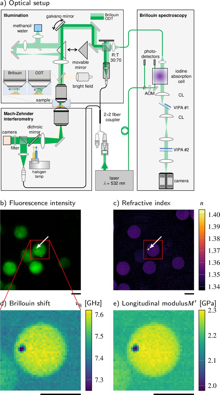
Correlative instrument and phantom measurements. The original panel lettering, scale bars and colour scales are retained.
Figure 1 from Correlative all-optical quantification of mass density and mechanics of subcellular compartments with fluorescence specificity. Raimund Schlüßler et al. eLife 11:e68490 (2022). © Schlüßler et al. 2022. DOI / source. Reproduced under CC BY 4.0. Complete figure; no content changes. Display size and image encoding may differ.
Open full-size figure ↗04 / Brillouin spectroscopy
Single-frequency operation is a starting point. The source must also stay spectrally clean and sufficiently stable during acquisition. A single spatial mode, a TEM00 beam or single-mode fiber delivery alone does not establish single-longitudinal-mode operation.
| Specify | Practical question |
|---|---|
| Wavelength | Does it suit sample absorption, detector sensitivity, optics and the available rejection or reference scheme? |
| Laser linewidth | Is it small compared with the sample line and the instrumental response? The 2025 consensus gives <100 MHz as a typical starting criterion; linewidth studies can require much tighter limits. |
| Drift and mode hops | What happens during a full map? Define warm-up, environmental conditions, lock access and the recalibration interval. |
| Spectral purity | What side modes and amplified spontaneous emission remain near the measured bands after filtering? A narrow main line alone is insufficient. |
| Delivered power and noise | What reaches the sample after all losses? Determine an exposure budget and measure power fluctuations in the relevant bandwidth. |
| Delivery and feedback | Specify beam size, polarization, coupling and isolation from back-reflections. Confirm the laser remains stable in the assembled optical path. |
Treat numerical criteria as a measurement-specific budget, not a universal product guarantee. In stimulated systems, include the relative frequency noise of the pump and probe and the detector’s noise floor. [1][2][8]
Compare single-frequency laser specifications05 / Brillouin spectroscopy
Bulk backscattering in hydrated samples usually probes a GHz longitudinal response. AFM indentation, tensile tests and rheology use different deformation modes and timescales. Converting between them needs a justified constitutive model; there is no universal conversion from Brillouin shift to low-frequency stiffness. [1][5]
Hydration can strongly affect Brillouin measurements. Refractive index, density, composition and temperature can also change the observed contrast. Compare matched conditions and use complementary measurements when claiming a specific material change. [5]
The adipocyte study below is a useful counterexample to reading a shift map as a stiffness map: lipid droplets have a higher Brillouin shift but a lower inferred longitudinal modulus than the surrounding cytoplasm once refractive index and density are included. [4]
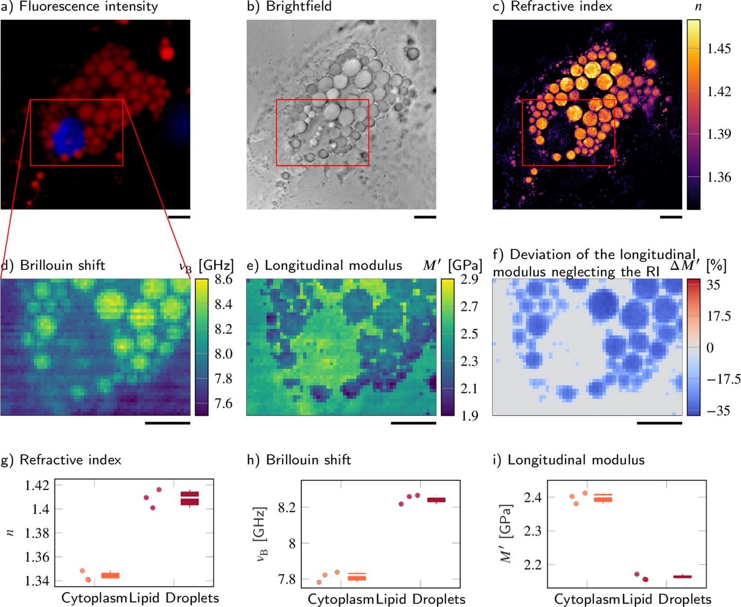
Published adipocyte measurements. Compare the Brillouin-shift map (d), derived longitudinal-modulus map (e), and the authors’ comparison plots (g–i). They show why optical and density information matter.
Figure 5 from Correlative all-optical quantification of mass density and mechanics of subcellular compartments with fluorescence specificity. Raimund Schlüßler et al. eLife 11:e68490 (2022). © Schlüßler et al. 2022. DOI / source. Reproduced under CC BY 4.0. Complete figure; no content changes. Display size and image encoding may differ.
Open full-size figure ↗High numerical aperture collects a range of scattering angles and can broaden spectra. Mixed sampling volumes can contain several materials or modes. Check whether apparent broadening reflects the sample’s damping, angular averaging or unresolved components before reporting viscosity. [8][10]
06 / Brillouin spectroscopy
Map acoustic contrast in cells, hydrogels and tissue; study spatial heterogeneity or responses to a controlled perturbation. Correlative fluorescence or chemical imaging helps identify the structures involved. [3][4]
Follow sound velocity and damping, relaxation, phase changes and elastic anisotropy. Temperature, pressure, polarization and scattering geometry become experimental variables. [1][9]
Probe confined and surface acoustic modes or phononic structures. Magnetic Brillouin scattering can interrogate spin waves; assigning a peak then requires the appropriate magnon model. [9]
The bulk longitudinal equations above do not describe every surface, confined, anisotropic or magnetic mode. Identify the mode and boundary conditions before calculating a modulus. [9]
07 / Brillouin spectroscopy
01
Choose shift, linewidth, a derived modulus or a spatial contrast. Record sample preparation, medium, temperature, geometry and polarization. Decide which independent measurements the interpretation needs.
02
Measure power at the sample and background from the chamber, substrate and optics. Test focus and aberrations at the intended depth. Keep illumination and collection geometry reproducible.
03
Measure a suitable reference at controlled temperature before and after a run. Establish the frequency scale, free spectral range, instrumental line shape and drift. Repeat controls through long maps.
04
Save raw frames or spectra and calibration data. Document background treatment, model, linewidth convention, instrument-response correction, uncertainties and failed-fit criteria. Inspect residuals and representative raw spectra.
05
Record sample power, dwell time, scan step, acquisition duration and repeat measurements. Test for heating or biological change at the chosen exposure; optical access alone does not guarantee a non-perturbing measurement.
06
Publish the shift and linewidth with their uncertainty. State the n, ρ and constitutive assumptions used for any derived mechanical quantity. Use matched controls and complementary methods for causal claims.
Practical workflow informed by the methods and reporting literature. [1][2][4][7][8][10]
SciPy curve_fit supports nonlinear least-squares fitting; supply a physically justified line model and appropriate uncertainties. h5py can store raw spectra, calibration, maps and metadata in HDF5. Both projects use permissive BSD licences: SciPy licence and h5py licence. These are general tools, not validated Brillouin analysis pipelines.
Archive units, software versions, fit settings and the original data alongside exported images. A colour map alone is insufficient to reproduce the analysis.
08 / Brillouin spectroscopy
The figures on this page are reproduced from the research papers identified in their captions. All three are covered by Creative Commons Attribution 4.0, which permits commercial redistribution with attribution, a licence link and an indication of changes. Their captions contain no separate third-party restriction.
Keep each figure’s attribution and licence notice when reusing it. Resizing and image encoding for web display do not change the scientific content. Reuse does not imply endorsement by the authors or publishers. The figure licences apply to those figures; other referenced papers retain their own terms.
Download the image attribution and licence record ↗Before you specify
 Raman spectroscopy
Stokes and anti-Stokes scattering, molecular fingerprints, depth resolution, and a complete microplastic mapping workflow with 3 interactive simulations.
Open guide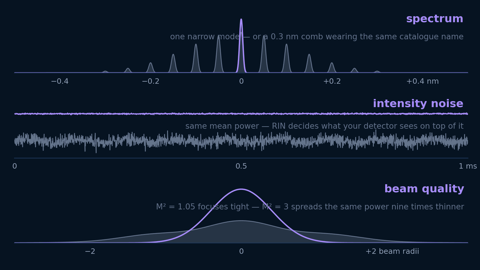 Photonics
Linewidth, spectral width, RIN, M², and coherence length answer five different questions. Translate each into the units your experiment is designed in — and learn which ones not to pay for.
Open guide Photonics
Why diode lasers drift or become noisy, how to identify the physical source of instability, and how to choose an appropriate stabilization architecture across 7 stability axes.
Open guide