Start from the ray geometry, not the catalog table
The grating maps wavelength to angle. The focusing optic maps angle to position. A slit or detector samples that position. Every useful performance number follows from those three operations.
Scanning monochromator
An entrance slit defines the source, the grating selects wavelength, and an exit slit transmits one finite band. Rotating the grating scans that band across a single-channel detector or uses the output as a tunable source. The measurement is sequential in wavelength.
Imaging spectrograph
The exit slit is replaced by an array at the focal surface. Many wavelengths are recorded at once, and the slit height may carry spatial information. Pixel pitch, sensor width and focal-plane aberrations become first-order specifications.
The crossed Czerny–Turner bench
A concave collimating mirror places the entrance slit at infinity, a plane reflection grating changes propagation angle according to wavelength, and a second concave mirror images the slit onto the exit plane. In a crossed layout the incident and diffracted arms cross in plan view, separating the ports while keeping the package compact. A nominally symmetric arrangement uses comparable incidence and diffraction angles and mirror conjugates; an asymmetric crossed arrangement deliberately uses unequal arm angles or conjugates to clear hardware, control anamorphic magnification, or optimize a wavelength range. Symmetry reduces some odd-order aberration terms but does not eliminate off-axis astigmatism.
Rotate the grating: the selected wavelength walks through the fixed exit slit. This is the scanning degree of freedom.
Derivation I
The grating equation
Let adjacent grooves be separated by d. With incidence angle α and diffraction angle β measured from the grating normal under the same-side sign convention, the path increment between rays from adjacent grooves is d sin α on arrival and d sin β on departure. Constructive interference requires the total phase increment to be an integer multiple of 2π:
Canceling 2π gives the reflection-grating equation:
m is the signed diffraction order; d is groove spacing; α and β follow the declared sign convention.
A different laboratory sign convention may show a minus sign. The physics is unchanged if the angles are used consistently. Groove density σ in lines per unit length is simply σ = 1/d.
Derivation II
Angular and linear dispersion
Hold the incidence angle fixed and differentiate the grating equation with respect to wavelength:
Angular dispersion increases with diffraction order and groove density, and grows as |β| approaches 90°.
At a focal length f, a small angular interval maps to dx ≈ f dβ. Therefore the linear dispersion is dx/dλ = mf/(d cos β), and its reciprocal—the catalog quantity in nm/mm—is:
Reciprocal linear dispersion is local, not universal. It changes with β across a scan; catalog values are normally quoted at a stated wavelength and grating, here 435.8 nm with 1200 g/mm.
Derivation III
Slit-limited bandpass
For equal entrance and exit slits of width w, approximately unit magnification and negligible aberration, convolution of their rectangular transmission functions produces a triangular line shape whose FWHM corresponds to one slit width at the focal plane. Thus:
This is the design equation requested most often: double focal length or groove density and the ideal slit contribution halves.
If the projected entrance-slit width is Mw and the exit slit differs, the support of the convolution spans D⁻¹(Mwin + wout); its FWHM is set by the wider projected slit. Quote entrance and exit widths separately whenever magnification or anamorphism is appreciable.
Where closing the slit stops helping
A grating illuminated across N grooves has resolving power R = mN. The corresponding diffraction-limited separation is:
N is the number of coherently illuminated grooves, not the total number ruled on the blank.
Real resolution should be treated as an instrument-function budget. If the separate terms are close to Gaussian, a useful engineering estimate is
This root-sum-square form is not an exact description of rectangular slits, but it correctly exposes the crossover: once slit broadening is below the quadrature sum of diffraction, aberration and sampling, closing the slit discards photons without materially narrowing the line. Measure the instrument line shape with a narrow calibration lamp at the intended wavelength and slit height.
Étendue is the budget that cannot be negotiated
Radiance is conserved by passive optics. A relay may trade beam area for solid angle, but it cannot compress an incoherent source into a smaller phase-space volume without losing light.
In a medium of refractive index n, the invariant is n²AΩ. In air, n ≈ 1 and the familiar AΩ form is sufficient.
For a small circular cone in air, NA ≈ 1/(2F) and Ω ≈ πNA² ≈ π/(4F²), where F is f-number. A slit of width w and illuminated height h therefore accepts, to first order, G ∝ wh/F². This is why slit height matters for an extended lamp even though it does not enter the one-dimensional dispersion equation.
The f-number mismatch trap
A fast source cone overfills a slower monochromator. For uniformly filled incoherent cones, the ideal angular acceptance fraction is approximately (Fsource/Fmono)². The rejected rays hit baffles, mirror cells or the housing; good baffling absorbs them, while imperfect baffling converts some fraction into wavelength-independent background and ghosts.
| Input cone | Into f/4.2 | Into f/6.5 | Experimental consequence |
|---|---|---|---|
| f/1.4 camera lens | ≈ 11% | ≈ 4.6% | Severe pupil overfill; use a relay that images the source and matches both pupil and slit. |
| NA 0.22 fibre (≈ f/2.27) | ≈ 29% | ≈ 12% | A bare fibre-to-slit placement throws away most modes; use a fibre coupler with the correct output f/#. |
Fractions assume a uniform radiance distribution and no focal-ratio degradation. Real multimode fibres often emerge faster than their nominal launch NA, so measure the far field when throughput matters.
Extended sources
An arc, filament or diffuse sample fills position and angle. Image the source onto the slit and the condenser pupil onto the grating. With a continuum, widening equal slits increases accepted spatial flux roughly linearly and bandpass linearly, so integrated background can scale approximately as w² until another aperture limits the system.
Point and single-mode sources
A diffraction-limited laser or single-mode fibre occupies low étendue. Choose magnification so the waist fits the slit while its transformed divergence fits the monochromator pupil. Opening the slit beyond the imaged waist gains no signal; it only admits alignment drift, scatter and background.
Bench rule: inspect two planes.
Verify the source image at the entrance slit and the pupil image at the grating. A bright slit image does not prove correct pupil fill, and a filled grating does not prove the slit is spatially matched.
Most false structure is generated after the sample
Astigmatism changes the spatial line image, higher orders create spectrally plausible impostors, and diffuse scatter creates a floor that no amount of detector dynamic range can recover.
Astigmatism
For an off-axis spherical mirror, tangential and sagittal rays have different effective focal lengths. The entrance slit may focus sharply in dispersion while its vertical image becomes a long sagittal smear. Fibre tracks then overlap even when spectral peaks remain apparently narrow.
Coma
Off-axis pupil zones have unequal transverse magnification, producing an asymmetric tail. Coma grows rapidly with aperture and field angle, biases peak centroids, and cannot be represented honestly by a single FWHM number.
Spherical aberration
Marginal and paraxial zones of a spherical mirror do not share a focus. Slower f/# reduces the error, but at the price of accepted solid angle. It becomes visible when slits are closed below the geometric blur floor.
Engineering response
Correct the focal plane when the slit height carries data
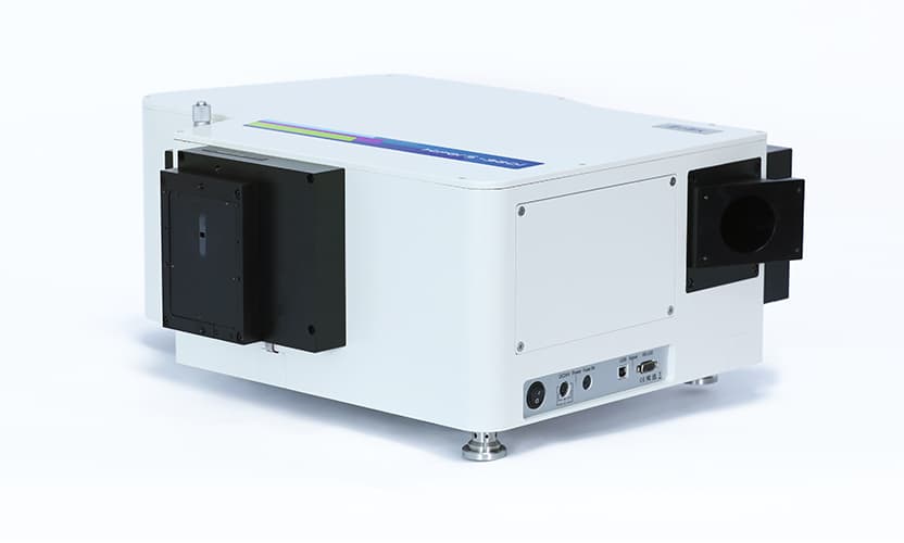
The HiperS-320i uses a full-focal-plane correction architecture with toroidal collimating and focusing surfaces, an on-axis triple-grating turret and automatic focusing. Different tangential and sagittal curvatures supply independent optical power in the two meridians, bringing the two line foci back together across a 29 × 14 mm focal plane. This is material for multi-fibre and multi-track measurements; it is not merely a prettier single spectrum.
Order overlap: a correct peak at the wrong wavelength
The grating only constrains the product mλ. Light at 400 nm in second order reaches the same diffracted angle as 800 nm in first order; 300 nm in third order also reaches that angle. The detector cannot infer which order produced a photon. Order sorting therefore belongs before the dispersive stage, where an automated long-pass wheel can track the scan.
Choose a cut-on above the unwanted λ/2 band but below the desired first-order wavelength, then verify transmission at the actual incidence angle.
A representative sequence uses an open position in the UV, a 320 nm cut-on once first-order scanning moves beyond roughly 640 nm, and a 610 nm cut-on beyond roughly 1220 nm. Those crossover points follow from 2λcut-on; they are not universal prescriptions. Lamp spectrum, filter edge, grating efficiency, third-order content and detector sensitivity must be checked together.
Stray light is an optical transfer path
Groove-placement errors and microroughness scatter light away from the ideal diffraction angle. Dust, fingerprints and damaged coatings add broad scatter. Zero-order reflections can strike baffles and re-enter the camera path; detector windows and filters create ghosts; a dispersed beam can reflect and encounter the grating again. These mechanisms scale differently with wavelength and slit setting, so a single rejection number should be treated as a test condition, not a universal background model.
| Architecture | Net dispersion | Catalog rejection class | Use it when |
|---|---|---|---|
| Single Czerny–Turner | One stage | ≈ 10⁻⁴ to 10⁻⁵ | Throughput and simplicity dominate; signal is not adjacent to an overwhelmingly bright line. |
| Additive double | Dispersions add; effective focal length doubles | 10⁻⁷ | Resolution is the bottleneck: 0.04 nm for 300Di or 0.025 nm for 500Di under stated test conditions. |
| Subtractive double | First-stage dispersion is canceled at the final output | 10⁻⁹ | Extreme rejection is required before a downstream analyzer, detector or sensitive sample. |
A necessary correction about subtractive mode
Dispersion is deliberately nonzero at the intermediate slit—that is where wavelength selection occurs. Opposite dispersion in the second stage makes the final output approximately non-dispersed. This cancels angular and spatial chirp, but it does not guarantee transform-limited ultrafast pulses: finite selected bandwidth lengthens a pulse, and grating group delay must still be measured or modeled.
Match the architecture to the dominant error term
The correct configuration is the shortest chain that suppresses the experiment's limiting background while preserving enough étendue to finish the measurement on a useful timescale.
APPLICATION 01
Tunable monochromatic source for responsivity, QE and IPCE
Physical principle
A continuum lamp is spectrally sliced, and the photon flux incident on the device under test is normalized to a calibrated reference photodiode. For IPCE, the measured photocurrent is converted to electrons per incident photon, not merely divided by optical power.
Optical challenge
Arc wander, lamp aging, wavelength-dependent grating efficiency and detector responsivity all masquerade as sample structure. A broad lamp also supplies exactly the short-wavelength photons that reappear as higher diffraction orders.
Optimal configuration
Use a xenon arc source when UV–visible radiance is required and QTH when red–NIR stability is more valuable. Image the arc or filament onto the entrance slit with an f/#-matched condenser; put the SD25 order-sorting wheel before the entrance slit; use an Omni-λ150 for legacy, compact broad-band systems or the faster f/3.5 Omni-λ200i for current throughput-limited builds. Split the exit beam only after spectral selection, and record the reference channel simultaneously.
APPLICATION 02
Photoluminescence and steady-state or time-resolved fluorescence
Physical principle
Excitation creates a non-equilibrium population; the spectrometer measures the radiative relaxation spectrum. Steady-state work estimates integrated spectral intensity, whereas time-resolved work measures the impulse response and therefore requires a pulsed source plus timing electronics or a frequency-domain modulation scheme.
Optical challenge
Fluorescence is weak, excitation leakage is bright, and the detector decision changes the entire noise model. A photon-counting PMT has essentially no read-noise penalty for a slow scan; a cooled InGaAs detector is required once silicon response collapses in the 0.8–1.7 µm band, but dark current and 1/f noise then matter.
Optimal configuration
Collect at 90° for clear solutions or in front-face geometry for absorbing and scattering samples. Place the excitation rejection filter before the entrance slit. Choose Omni-λ200i for broad weak bands, Omni-λ300i for the usual resolution/throughput compromise, or HiperS-320i when a fibre bundle or multiple spatial tracks must remain separated. Use photon counting for a PMT chain; use a chopper plus lock-in for an analog detector chain. These are alternative estimators, not accessories to stack indiscriminately.
APPLICATION 03
Ultra-low stray-light Raman and Rayleigh-edge rejection
Physical principle
A Raman shift Δν̃ produces a wavelength displacement that is approximately Δλ ≈ λ₀²Δν̃ for small Stokes shifts when λ₀ is expressed in consistent units. At 532 nm, 50 cm⁻¹ is only about 1.42 nm from the laser; at 785 nm it is about 3.08 nm.
Optical challenge
The elastically scattered field can exceed a low-wavenumber Raman line by many orders of magnitude. Closing a slit narrows the instrumental profile but does not remove grating scatter wings, housing reflections or detector blooming. A nominal edge-filter transition is also not the same thing as measured system rejection at the sample plane.
Optimal configuration
Use a clean single-frequency laser, spatial filtering, a high-OD edge or volume-holographic filter, and a subtractive Omni-λ300D/500D pair (current datasheet codes: 300Di/500Di) as a tunable prefilter where 10⁻⁹-class catalog rejection is required. The subtractive pair cancels net angular/spatial dispersion at its final output, so an analyzing spectrograph may follow. For routine Raman farther from the line, a single Omni-λ300i is usually more photon-efficient; for the most demanding low-shift work, a purpose-built triple stage is the safer architecture.
APPLICATION 04
Transmission and high-optical-density filter characterization
Physical principle
Optical density is OD = −log₁₀(T), with T = (Iₛ − Iₛ,dark)/(Iᵣ − Iᵣ,dark) after reference and dark correction. OD 6 and OD 8 correspond to transmissions of 10⁻⁶ and 10⁻⁸, respectively.
Optical challenge
Detector bit depth is not system dynamic range. Dark current, drift, ghost reflections, pinholes, source scatter and wavelength leakage establish a false transmission floor. At OD 8, one nanowatt of out-of-band leakage accompanying a 0.1 W equivalent reference can dominate the result.
Optimal configuration
Use a source monochromator plus order sorting, monitor the incident beam, place the filter at the specified angle and polarization, and analyze the transmitted light with a second monochromator or a subtractive Omni-λ300D/500D pair (300Di/500Di in the current datasheet). Establish the floor with a beam block, verify linearity with traceable neutral-density steps, and change detector gain or integration time in overlapping ranges. A 10⁻⁹ stray-light specification makes OD 8 plausible; it does not certify OD 8 by itself.
APPLICATION 05
Plasma emission and high-resolution line diagnostics
Physical principle
Electron temperature, density, species concentration and flow are inferred from line ratios, Stark widths, Doppler widths and wavelength shifts. The instrument function must be narrower than the physical feature being fitted, or it must be independently measured and deconvolved.
Optical challenge
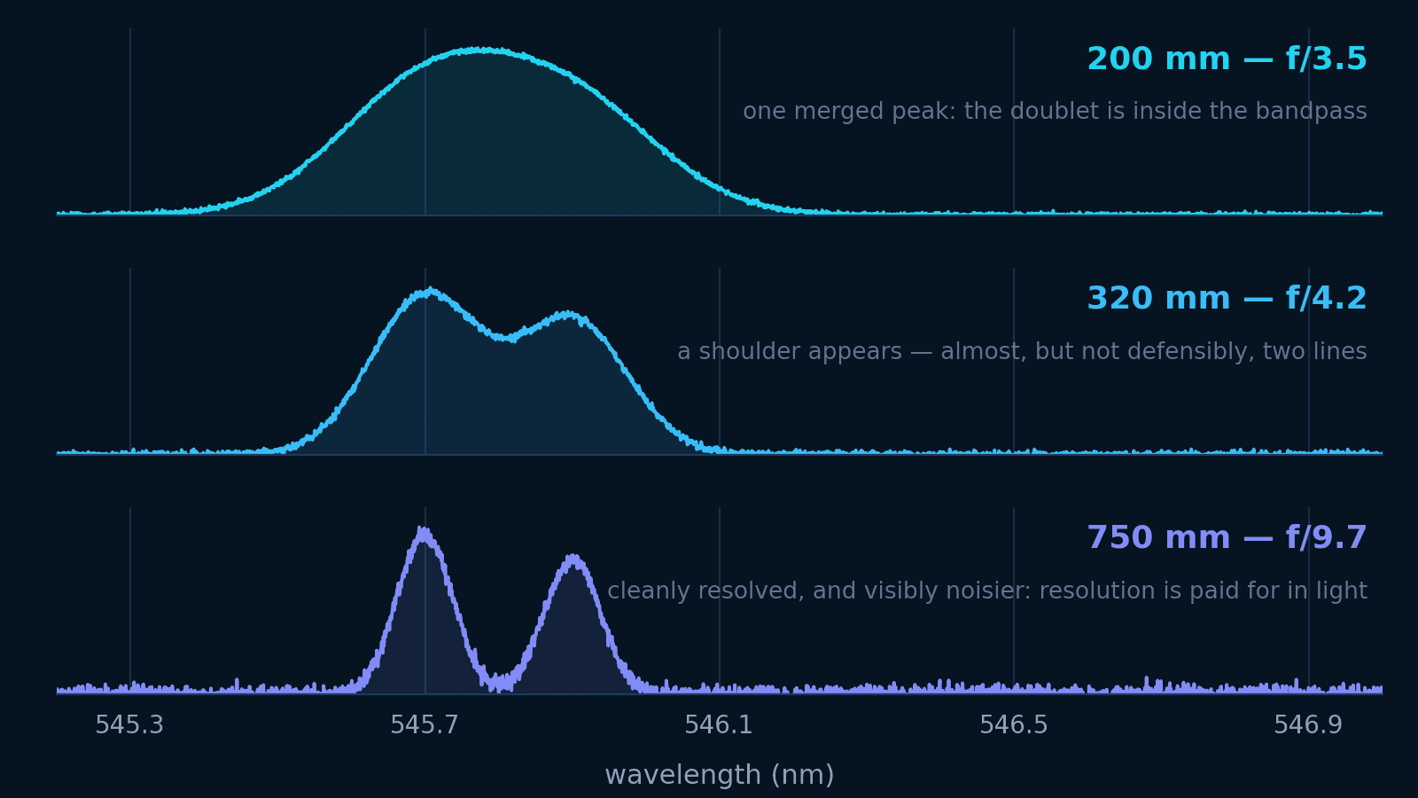
Lines separated by less than 0.05 nm demand fine reciprocal dispersion, stable wavelength calibration and a narrow effective slit image, while plasma continua and shot-to-shot fluctuations favor simultaneous array detection. Fibre bundles add a spatial-imaging requirement that a conventional astigmatic spectrograph may not meet.
Optimal configuration
Pair an 1800–2400 g/mm grating with the Omni-λ500i or Omni-λ750S/750i class. Near normal incidence, a 25 µm slit with 1800 g/mm and f = 500 mm gives an ideal slit contribution of about 0.028 nm; a 25 µm slit with 2400 g/mm and f = 750 mm gives about 0.014 nm before aberration, pixel and diffraction terms. Use HiperS-320i instead when preserving multiple fibre images is more important than maximum dispersion.
Choose the shortest focal length that closes the resolution budget
Longer focal length reduces reciprocal linear dispersion, but its slower aperture costs photons. Move to a double stage for a demonstrated rejection or resolution requirement—not as a default upgrade.
| Model | Focal length | f/# | Reciprocal dispersion¹ | Accuracy¹ | Repeatability¹ | Stray light | Exit / detector flexibility | Primary fit |
|---|---|---|---|---|---|---|---|---|
| Omni-λ150 (legacy) | 150 mm | f/4.2 | 5.4 nm/mm | ±0.25 nm | ±0.1 nm | Not stated in legacy sheet | Model-dependent; dual-grating platform | Compact tunable sources, broadband transmission and responsivity work |
| Omni-λ200i | 200 mm | f/3.5 | 3.58 nm/mm | ±0.2 nm | ±0.1 nm | 5 × 10⁻⁵ | Slit and/or CCD variants; dual grating turret | Weak broad bands, lamp monochromation, routine UV–Vis |
| Omni-λ300i | 320 mm | f/4.2 | 2.29 nm/mm | ±0.2 nm | ±0.025 nm | 1 × 10⁻⁵ | Single/dual slit or CCD combinations; triple turret | General Raman, PL, fluorescence and detector calibration |
| Omni-λ500i | 500 mm | f/6.5 | 1.49 nm/mm | ±0.2 nm | ±0.025 nm | 1 × 10⁻⁵ | Single/dual slit or CCD combinations; triple turret | Resolved emission structure, laser spectra and line diagnostics |
| Omni-λ750S / 750i† | 750 mm | f/9.7 | 1.02 nm/mm | ±0.2 nm | ±0.025 nm | 1 × 10⁻⁵ | Single/dual slit or CCD combinations; triple turret | Atomic/plasma lines and known sub-0.05 nm requirements |
| HiperS-320i | 320 mm | f/4.4 | 2.29 nm/mm | ±0.2 nm | ±0.025 nm | 5 × 10⁻⁵ | Up to two entrances/two exits; on-axis triple turret | Multi-track, multi-fibre, LIBS and focal-plane imaging |
| Omni-λ300D / 500D (300Di / 500Di)‡ | 640 / 1000 mm additive; 320 / 500 mm subtractive | f/4.2 / f/6.5 | 1.15 / 0.75 nm/mm additive; 2.29 / 1.49 subtractive | ±0.2 nm | ±0.025 nm | 10⁻⁷ additive; 10⁻⁹ subtractive | Entrance, 24 mm motorized middle slit, final slit/detector coupling | High resolution in additive mode; Raman/OD filtering in subtractive mode |
¹ Current Omni-λ200i/300i/500i/750i and HiperS values are manufacturer test data at 1200 g/mm and 435.8 nm. Dispersion is local. Double-stage values are additive/subtractive pairs from the corresponding datasheet.
† “Omni-λ750S” remains in some Precisometer ordering and application material; the current source datasheet supplied with this catalog uses “Omni-λ750i.” Confirm the exact suffix and acceptance values on the quotation.
‡ “Omni-λ300D/500D” describes the double-monochromator families; the linked current manufacturer datasheet identifies the orderable series as Omni-λ300Di and Omni-λ500Di.
Omni-λ150 is a legacy 150 mm platform and is not part of the current 200/320/500/750 mm i-series datasheet. Its row is retained because installed systems and tunable-source literature still use it.
PMT exit slit
Best when a sequential scan, very low photon rate and flexible detector chemistry matter. Bandpass is set by both slits; wavelength dwell time can be optimized point by point.
CCD / sCMOS focal plane
Best for transient or unstable spectra and simultaneous coverage. Require at least 2–3 pixels per measured resolution element and verify focus across the detector height.
Dual exit ports
Useful when the same bench must alternate between photon-counting scans and array acquisition. Specify the port selector, both flange standards and whether recalibration follows a switch.
Turn the measurement into an orderable optical system
Write the acceptance test before selecting the model. “High resolution” and “low stray light” are not specifications; two separable lines, a rejection ratio at a stated offset, and a minimum detected flux are.
- 1
Define the measurand and the smallest spectral feature.
State wavelength range, closest line separation, required centroid precision, signal level, allowed acquisition time and the background that must be rejected. Convert Raman cm⁻¹ to nm at the actual excitation wavelength.
- 2
Allocate the resolution budget.
Reserve terms for source linewidth, entrance/exit slit image, diffraction, aberration, detector pixels and calibration drift. A defensible first pass gives the monochromator no more than roughly half the required feature spacing.
- 3
Solve for the slit width, then check whether it is physical.
Using the local catalog dispersion, w ≈ Δλtarget/D⁻¹. For Δλtarget = 0.10 nm on an Omni-λ300i at 2.29 nm/mm, w ≈ 44 µm. If this falls below the measured aberration floor or two detector pixels, change focal length or groove density instead of closing farther.
- 4
Choose groove density before blaze wavelength.
Groove density must satisfy dispersion and coverage. Then select a blaze near the signal band and inspect the efficiency curve for polarization and order. A blaze label is not an efficiency guarantee across the entire scan.
- 5
Build a turret around distinct jobs.
A practical triple turret often carries a 300 or 600 g/mm survey grating, a 1200 g/mm analytical grating and an 1800 or 2400 g/mm high-resolution grating. Replace any slot whose blaze or scan limit misses the real experiment; the turret is not a collector’s set.
- 6
Match source image, pupil and detector.
Specify fibre NA or relay f/#, slit height, source-image magnification, grating footprint, camera pixel pitch and active width. Include focal-ratio degradation for multimode fibre and a focus check across the complete array.
- 7
Specify order sorting and coatings by wavelength band.
List filter-wheel transition wavelengths and safe overlap intervals. Choose UV, aluminum, protected-silver or gold optics from measured reflectance in the band—not from a generic “broadband” description.
- 8
Choose manual or motorized slits from the measurement protocol.
Manual slits suit fixed, alignment-stable experiments. Motorized slits are justified when software changes bandpass, throughput must be repeated across many scans, or remote operation matters. Acceptance-test actual width repeatability and backlash.
- 9
Define calibration and rejection tests.
Specify calibration lamps, line wavelengths, warm-up time, scan direction, slit widths, detector gain, environmental conditions and the wavelength offset at which stray light is tested. Record an instrument function, dark spectrum and blocked-beam floor.
- 10
Freeze interfaces before purchase.
Document optical-axis height, port orientation, flange, shutter, filter wheel, detector cooling envelope, cable clearance, controller interface and software driver. The optically correct instrument can still be unusable if the selected port collides with the bench.
Configuration handoff
Carry the calculation into a real turret and port layout
Use the Turret Planner to check groove density, blaze and wavelength coverage, then pass the result to the Monochromator Builder for focal length, coating, entrance, slit mechanism and PMT/array exit ports. For unusual source étendue, tall fibre bundles, deep-UV coatings or OD/Raman rejection targets, send the full optical budget to Precisometer's application physicists for custom ray tracing and aperture matching.