Laser application guide
Designing a confocal fluorescence excitation system
Begin with the fluorophores and specimen. Then connect wavelength, sample-plane power, pinhole, spatial sampling, modulation, and fiber delivery into one imaging budget.
Section, don’t flood
A focused spot and conjugate pinhole reject much of the out-of-focus fluorescence.
Specify at the sample
Power after every delivery and scanning loss is the useful excitation quantity.
Synchronize every line
Blanking, power setpoint, scanner position, detector gate, and acquisition share one timing chain.
The decision in one sentence
Optimize information per photon—not laser power in isolation.
Confocal microscopy trades photons for optical sectioning. The excitation focus limits where fluorescence is created, and the detection pinhole limits which emitted photons are accepted. The useful source is therefore the one that delivers the right wavelength and controllable power into the scanner, with enough speed and stability to preserve contrast over an entire image or Z-stack.
Define the labels
Map each excitation spectrum to an emission band, detector, and acceptable cross-excitation.
Define the image
Objective NA, optical section, field, pixel pitch, Z step, and temporal resolution.
Close the dose budget
Power at the specimen, dwell, averaging, revisit rate, and tolerated bleaching or phototoxicity.
1 · Confocal signal path
Two aligned foci create the optical section.
“Confocal” means the illumination focus and detection aperture are conjugate to the same point in the specimen. Scanning that point builds a two-dimensional image; shifting focus in Z builds a volume.
Laser
Stable wavelength and controlled power
Modulator
Blanking and intensity setpoint
Scanner
Raster or parallel illumination
Objective
Focus excitation into the sample
Pinhole
Reject defocused emission
Detector
Convert accepted photons to signal
The excitation point-spread function determines where fluorescence is generated.
The detection point-spread function and pinhole determine which photons are accepted.
Point scanning
One diffraction-limited point is rastered through the field.
Strength: Flexible pinhole, spectral detection, and precise region control.
Laser consequence: Fast analog or TTL blanking keeps light off the sample during flyback and inactive pixels.
Line scanning
A focused line is imaged onto a slit or camera detector.
Strength: Higher acquisition speed with partial optical sectioning.
Laser consequence: Uniformity along the line and synchronization with the camera become source-and-optics requirements.
Spinning disk
Many pinholes illuminate and detect multiple points in parallel.
Strength: Fast, gentle imaging for dynamic samples and live cells.
Laser consequence: Coupling efficiency, field uniformity, and power across many simultaneous spots matter more than peak power.
2 · Pinhole + optical sectioning
The pinhole is a signal–sectioning control.
A smaller detection aperture rejects more defocused light, but also blocks useful emission. Its physical diameter is commonly normalized in Airy units so the setting follows wavelength, numerical aperture, and magnification.
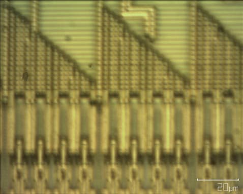
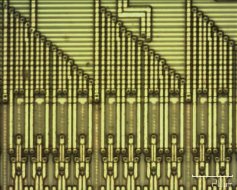
Airy-unit diameter at the pinhole
- λem
- representative emission wavelength
- M
- sample-to-pinhole magnification
- NA
- objective numerical aperture
- dAU
- diameter corresponding to 1 Airy unit
Use the actual relay magnification to the pinhole plane. Objective magnification alone is only a proxy when additional optics change the scale.
Sharper section, lower signal
Useful when background dominates and photon budget allows it.
Balanced starting point
A common compromise between optical sectioning and detected fluorescence.
More signal, less sectioning
Useful for dim or fast samples when contrast can tolerate more background.
3 · Excitation channels
Choose lines from the complete spectral panel.
An excitation peak is not a command. The correct line balances excitation efficiency, cross-excitation, dichroics, emission windows, detector response, and the exposure tolerance of every label in the specimen.
405 nm
Violet channel
Common for blue-emitting nuclear stains and selected violet-excited probes.
Short wavelengths can be phototoxic; minimize exposure and check objective and fiber transmission.
488 nm
Blue channel
A widely used excitation line for green fluorescent protein and fluorescein-class labels.
Often the busiest channel, so modulation speed, noise, and power after the fiber deserve special attention.
532 / 561 nm
Green–yellow channel
Useful for many orange-red fluorophores; 561 nm often provides a cleaner excitation match than 532 nm.
Choose from the measured excitation spectrum and filter set, not from laser availability alone.
637 / 640 nm
Red channel
Common for far-red labels and multicolor panels that need more spectral separation.
Confirm detector quantum efficiency and chromatic registration at the long-wavelength end of the system.
Close the power budget per channel. Record output at the laser, after the combiner or fiber, and at the specimen plane. Dichroic transmission, AOTF/AOM efficiency, scanner coatings, objective transmission, and fiber coupling can make the weakest delivered channel different from the weakest laser head.
4 · Pinhole + sampling calculator
Connect the optics to the pixel grid and frame time.
Change the emission wavelength, objective, pinhole, field, pixel count, and dwell time. The estimates show why a nominal resolution target, detector aperture, sampling plan, and acquisition speed must be designed together.
Set the optical train
Confocal design lab
Illustrative starting points only; presets update every control.
First-order estimates
The calculated pitch is 0.195 µm; the model target is ≤ 0.075 µm. Your setting is 2.59× that target.
A balanced starting range for sectioning and signal collection.
Engineering estimates use dAU = 1.22 λemM/NA, 0.61 λem/NA as a widefield Rayleigh reference, and 0.4 λem/NA as an idealized small-pinhole confocal lateral estimate. The frame time excludes line flyback, averaging, bidirectional timing errors, and stage motion. Measure the point-spread function and effective magnification on the real system.
5 · Source architecture
The scanner determines how the laser must behave.
A good wavelength match is only the beginning. Confocal imaging exposes the sample point by point, so modulation edges, residual “off” light, noise, and channel registration can become visible image artifacts.
Individual laser modules
A direct route when the fluorescence panel is stable. Each wavelength can be independently serviced, attenuated, and modulated.
Qualify: Beam height, divergence, polarization, modulation input, warm-up, pointing stability, and spectral cleanup.
Multi-line fiber combiner
Combining channels into one single-mode delivery fiber simplifies alignment and makes the spatial mode repeatable at the microscope input.
Qualify: Power after the output fiber, channel isolation, connector and fiber type, per-line modulation, and output collimation.
Integrated confocal system
A system-level package couples excitation, scanning, collection, detection, and acquisition around a defined sample and workflow.
Qualify: Objective, field and Z range, detector bands, image rate, software interface, environmental control, and service boundary.
Modulation
Request rise/fall time, extinction ratio, latency, linearity, and the maximum usable frequency—not merely “TTL/analog available.”
Noise
Match the relative-intensity-noise measurement band to pixel and line times. Slow drift and fast noise create different image artifacts.
Spatial mode
A stable TEM00 or single-mode-fiber output supports repeatable focusing and channel overlap at the scan head.
Polarization
AOTFs, dichroics, fibers, and scanners can be polarization sensitive. Specify orientation and extinction where it affects throughput.
6 · Relevant products
Product starting points for confocal excitation.
These are live catalog entries that cover complete systems, multi-line delivery, microscopy integration, and a compact single channel. Final selection still depends on the fluorophore panel and power after the microscope optics.
Integrated application system
Confocal Laser Scanning Microscopy
A catalog starting point for a confocal microscope built around the laser source, scanning optics, detection, and data acquisition as one measurement chain.
- Confocal microscope architecture
- Laser + acquisition integration
- Free-space or fiber-coupled source options
Multi-channel source
Multi-wavelength SM Fiber Output Laser
A configurable multi-wavelength source for feeding several excitation channels through a shared single-mode spatial output.
- Multi-wavelength configuration
- Single-mode fiber output
- Shared microscope input path
Microscopy light engine
Microscopic Imaging Laser
A multi-line laser configuration intended for microscopic imaging, useful when compact channel control and system integration are the main design goals.
- Microscopy-oriented source
- Multi-line operation
- Configurable integration
Compact violet channel
MDL-XS-405
A compact 405 nm CW source for adding a violet excitation channel where a near-TEM00 beam and integrated electronics fit the instrument architecture.
- 405 nm CW output
- 1–200 mW catalog range
- Near-TEM00 beam
Need a 405 / 488 / 561 / 640 nm combiner?
Build the enquiry around delivered power per line, output fiber, modulation bandwidth, extinction ratio, connector, and control interface.
7 · Specification checklist
Send an imaging brief, not a wavelength list.
These inputs let the source, delivery, scanner, and detector be reviewed as one instrument.
Fluorophores
Excitation and emission spectra, brightness, photostability, and required channel order.
Power at sample
Useful range after fiber, collimator, scanner, dichroics, objective, and any AOTF/AOM.
Channel control
Independent enable, analog setpoint, TTL blanking, rise/fall time, and safe default state.
Delivery
Free space, SM or PM fiber, connector, numerical aperture, output collimation, and polarization.
Image geometry
Objective NA, sample-to-pinhole magnification, pinhole range, field, pixels, Z step, and working distance.
Acquisition
Pixel dwell, line/frame rate, averaging, bidirectional scanning, trigger polarity, and clock source.
Stability
Warm-up, short- and long-term power stability, pointing, RIN band, and channel-to-channel registration.
Sample constraints
Live or fixed, tolerated dose, motion timescale, refractive-index mismatch, and environmental control.
Application review
Bring one representative fluorophore panel and image sequence.
We can translate it into excitation lines, delivered-power ranges, fiber delivery, modulation, and the system questions that remain open.
8 · Common questions
Short answers before the design review.
Why does a confocal microscope use a pinhole?+
The detection pinhole is conjugate to the illuminated focal point. It preferentially passes light from that plane and blocks much of the defocused light, improving optical sectioning and contrast in thick or fluorescent samples.
Is a smaller pinhole always better?+
No. Closing the pinhole can improve sectioning and approach the ideal confocal point-spread function, but it also discards fluorescence and lowers signal-to-noise. Around one Airy unit is a practical starting point, then the sample and detector noise decide the optimum.
How much laser power should reach the sample?+
Only enough to achieve the required signal-to-noise within the permitted dwell time. Specify a controllable range at the specimen plane, measure it through the selected objective, and validate photobleaching or phototoxicity on the actual sample.
Do all channels need the same output power?+
No. Fluorophore cross-section, labeling density, optical throughput, detector sensitivity, and exposure budget differ by channel. Equal power at the combiner output rarely creates equal signal or equal photodamage.
When is single-mode fiber delivery useful?+
It provides a clean, repeatable spatial mode and can simplify alignment into the scanner. The tradeoff is coupling loss and a power budget that must be specified after the output fiber, not only at each laser head.
Research basis
This guide is an engineering overview. The optical sectioning, resolution, pinhole, and exposure discussions draw on representative primary studies:
- 1. Brakenhoff, Blom & Barends, “Confocal scanning light microscopy with high aperture immersion lenses,” Journal of Microscopy 117, 219–232 (1979).
- 2. Gu, Gan & Sheppard, “Three-dimensional coherent transfer functions in fiber-optical confocal scanning microscopes,” JOSA A 8, 1019–1025 (1991).
- 3. Gauderon & Sheppard, “Effect of a finite-size pinhole on noise performance in single-, two-, and three-photon confocal fluorescence microscopy,” Applied Optics 38, 3562–3565 (1999).
- 4. Hoebe et al., “Controlled light-exposure microscopy reduces photobleaching and phototoxicity in fluorescence live-cell imaging,” Nature Biotechnology 25, 249–253 (2007).
Continue exploring